Preparation is the key to success in any interview. In this post, we’ll explore crucial Advanced Math and Physics interview questions and equip you with strategies to craft impactful answers. Whether you’re a beginner or a pro, these tips will elevate your preparation.
Questions Asked in Advanced Math and Physics Interview
Q 1. Explain the concept of eigenvalues and eigenvectors.
Eigenvalues and eigenvectors are fundamental concepts in linear algebra. Imagine a linear transformation as a function that stretches, shrinks, or rotates a vector. Eigenvectors are special vectors that, when this transformation is applied, only change in scale; they don’t change direction. The factor by which they scale is the eigenvalue.
More formally, for a square matrix A and a non-zero vector v, if Av = λv, then λ is an eigenvalue and v is the corresponding eigenvector. The eigenvalue represents the scaling factor, and the eigenvector represents the direction that remains unchanged under the transformation.
Example: Consider the matrix A = [[2, 0], [0, 3]]. If we apply this matrix to the vector v = [1, 0], we get Av = [2, 0] = 2v. Thus, 2 is an eigenvalue, and [1, 0] is the corresponding eigenvector. Similarly, 3 is an eigenvalue with eigenvector [0, 1]. Eigenvalues and eigenvectors are crucial in various applications, including solving differential equations, analyzing stability of systems, and dimensionality reduction in machine learning.
Q 2. Describe the Schrödinger equation and its significance.
The Schrödinger equation is a fundamental equation in quantum mechanics that describes how the quantum state of a physical system changes over time. It’s analogous to Newton’s second law (F=ma) in classical mechanics, but instead of predicting the trajectory of a particle, it predicts the evolution of a wave function.
The time-dependent Schrödinger equation is given by: iħ ∂Ψ/∂t = ĤΨ, where:
iis the imaginary unitħis the reduced Planck constantΨ(psi) is the wave function, a complex-valued function describing the quantum state∂Ψ/∂tis the partial derivative of the wave function with respect to timeĤ(H-hat) is the Hamiltonian operator, representing the total energy of the system.
Solving the Schrödinger equation allows us to calculate the probabilities of different outcomes when we measure properties of a quantum system, such as energy or momentum. The equation’s significance lies in its ability to accurately predict the behavior of atoms and subatomic particles, leading to advancements in various fields like semiconductor physics, materials science, and nuclear technology. For stationary states, where the energy is constant, we use the time-independent Schrödinger equation, simplifying the calculation considerably.
Q 3. What are the different types of partial differential equations and their applications?
Partial differential equations (PDEs) are equations involving partial derivatives of a function with multiple variables. They are classified based on their order and type. The order is determined by the highest-order derivative. The type is determined by the characteristics of the equation. Common types include:
- Elliptic PDEs: These describe steady-state phenomena, like the steady-state temperature distribution in a solid. Laplace’s equation (∇²u = 0) is a prime example. Applications include electrostatics and fluid dynamics in steady states.
- Parabolic PDEs: These model diffusion and heat transfer processes. The heat equation (∂u/∂t = α∇²u) is a classic example. Applications include weather forecasting and heat treatment of materials.
- Hyperbolic PDEs: These describe wave phenomena, like sound waves or electromagnetic waves. The wave equation (∂²u/∂t² = c²∇²u) is a typical example. Applications include acoustics, seismology, and electromagnetism.
Other types, such as mixed-type PDEs, can exhibit characteristics of multiple categories. The choice of solution methods depends heavily on the type of PDE and boundary conditions. For example, Finite Element Method (FEM) is widely used for elliptic problems, while Finite Difference Method (FDM) is commonly used for parabolic and hyperbolic problems.
Q 4. Explain the concept of statistical significance and hypothesis testing.
Statistical significance assesses the probability of observing a result as extreme as, or more extreme than, the one obtained, assuming a null hypothesis is true. The null hypothesis is a statement that there is no effect or relationship between variables. Hypothesis testing is a formal procedure used to decide whether to reject or fail to reject the null hypothesis based on sample data.
We typically use a p-value to determine statistical significance. The p-value is the probability of obtaining the observed results (or more extreme results) if the null hypothesis were true. A small p-value (typically below a significance level, often 0.05) indicates that the observed result is unlikely to have occurred by chance alone, leading to rejection of the null hypothesis. This signifies that there is statistically significant evidence to support an alternative hypothesis (e.g., a difference between groups or a relationship between variables).
Example: Suppose we test a new drug’s effectiveness. The null hypothesis is that the drug has no effect. If the p-value from the analysis is 0.01, this suggests there is only a 1% chance of observing the obtained results (or more extreme) if the drug were truly ineffective. We would then reject the null hypothesis and conclude that the drug is statistically significantly effective.
Q 5. Derive the equation for the motion of a simple pendulum.
Let’s derive the equation of motion for a simple pendulum. We’ll use Newton’s second law and make some simplifying assumptions: the pendulum bob is a point mass, the string is massless and inextensible, and there’s no air resistance.
Consider a pendulum bob of mass m attached to a string of length L. Let θ be the angle the string makes with the vertical. The restoring force acting on the bob is the component of gravity along the tangential direction, which is -mg sin θ.
Applying Newton’s second law (F = ma) in the tangential direction, we get:
m (d²s/dt²) = -mg sin θ
where s is the arc length along the circular path. Since s = Lθ, we have d²s/dt² = L (d²θ/dt²). Substituting this into the equation, we get:
mL (d²θ/dt²) = -mg sin θ
Simplifying, we obtain:
(d²θ/dt²) = -(g/L) sin θ
This is the exact equation of motion. For small angles (θ ≈ 0), we can use the small-angle approximation sin θ ≈ θ, which simplifies the equation to:
(d²θ/dt²) = -(g/L) θ
This is a simple harmonic oscillator equation, with a period T = 2π√(L/g).
Q 6. How would you solve a system of linear equations using matrix methods?
Solving a system of linear equations using matrix methods is efficient and elegant. Consider a system of n linear equations with n unknowns, which can be represented in matrix form as Ax = b, where:
Ais ann x ncoefficient matrixxis ann x 1column vector of unknownsbis ann x 1column vector of constants
Several methods can solve for x:
- Gaussian elimination: This method systematically eliminates variables to transform the augmented matrix
[A|b]into row echelon form. Back substitution then yields the solution. - LU decomposition: This method factorizes matrix
Ainto a lower triangular matrixLand an upper triangular matrixU, such thatA = LU. The system then becomesLy = bandUx = y, which are easily solved by forward and backward substitution respectively. This is very efficient for multiple systems with the same coefficient matrixAbut differentb. - Inverse matrix method: If the matrix
Ais invertible, the solution is given byx = A⁻¹b. However, this method can be computationally expensive for large matrices.
The choice of method depends on factors like the size of the system, the properties of the matrix A (e.g., sparsity), and computational resources available. Libraries like NumPy in Python provide efficient functions for matrix operations, making these methods readily applicable.
Q 7. Explain the concept of Fourier transforms and their applications in signal processing.
The Fourier transform is a mathematical tool that decomposes a function into its constituent frequencies. Imagine a musical chord: it’s composed of different notes (frequencies) played simultaneously. The Fourier transform effectively separates these notes, revealing the amplitude and phase of each frequency component.
For a function f(t), its Fourier transform F(ω) is defined as:
F(ω) = ∫_{-∞}^{∞} f(t)e^(-iωt) dt
where ω represents angular frequency. The inverse Fourier transform recovers the original function from its frequency components:
f(t) = (1/2π) ∫_{-∞}^{∞} F(ω)e^(iωt) dω
Applications in signal processing are vast:
- Spectral analysis: Identifying the frequency components of a signal (e.g., audio signals, seismic data).
- Filtering: Removing unwanted frequencies from a signal (e.g., noise reduction).
- Signal compression: Representing a signal efficiently by keeping only significant frequency components (e.g., JPEG image compression).
- Signal deconvolution: Removing the effects of a blurring function from a signal (e.g., image deblurring).
The Fast Fourier Transform (FFT) is a computationally efficient algorithm for computing the discrete Fourier transform, making it widely used in digital signal processing applications.
Q 8. Describe the principles of quantum mechanics.
Quantum mechanics is a fundamental theory in physics that provides a description of the physical properties of nature at the scale of atoms and subatomic particles. Unlike classical mechanics, which describes the world at larger scales, quantum mechanics relies on probabilities and wave functions to describe the behavior of particles. At its core, it rests on several key principles:
- Quantization: Certain physical properties, like energy and angular momentum, can only take on discrete values, rather than a continuous range. Think of it like a staircase, where you can only stand on specific steps, not in between them. This is in contrast to a ramp in classical mechanics where you can be at any position.
- Wave-particle duality: Particles, like electrons and photons, exhibit properties of both waves and particles. This means they can diffract like waves (think of ripples in water) and also behave like discrete particles in some interactions.
- Probability and the Uncertainty Principle: We can only predict the probability of finding a particle in a particular state, not its exact position and momentum simultaneously. Heisenberg’s Uncertainty Principle quantifies this limitation: the more precisely we know a particle’s position, the less precisely we know its momentum, and vice versa.
- Superposition: A quantum system can exist in multiple states simultaneously until measured. Imagine a coin spinning in the air – it’s neither heads nor tails until it lands. Once measured, the system collapses into a single definite state.
- Entanglement: Two or more particles can be linked together in such a way that they share the same fate, regardless of the distance separating them. Measuring the state of one instantly determines the state of the others.
Quantum mechanics has revolutionized our understanding of the universe, leading to technological advancements like lasers, transistors, and nuclear magnetic resonance (NMR) imaging.
Q 9. What are the different types of probability distributions and their applications?
Probability distributions describe the likelihood of different outcomes of a random variable. Several types exist, each suited to different applications:
- Normal (Gaussian) Distribution: This bell-shaped curve is ubiquitous, modeling many natural phenomena like human height or measurement errors. It’s characterized by its mean (average) and standard deviation (spread). The Central Limit Theorem highlights its importance; the sum of many independent random variables tends towards a normal distribution, regardless of their individual distributions.
- Binomial Distribution: This distribution describes the probability of getting a certain number of successes in a fixed number of independent Bernoulli trials (experiments with two outcomes, like coin flips). It’s used in quality control and opinion polls.
- Poisson Distribution: This describes the probability of a given number of events occurring in a fixed interval of time or space, when these events occur independently and at a constant average rate. Examples include the number of cars passing a point on a highway per hour or the number of customers arriving at a shop per minute.
- Exponential Distribution: This describes the time between events in a Poisson process. It’s commonly used in reliability analysis, modeling the lifetime of components.
- Uniform Distribution: This distribution assigns equal probability to all outcomes within a specified range. It’s used in simulations and random number generation.
Choosing the correct probability distribution depends heavily on the problem at hand. Understanding their properties is crucial for statistical analysis, risk assessment, and modeling various real-world scenarios.
Q 10. Explain the concept of Lagrangian and Hamiltonian mechanics.
Lagrangian and Hamiltonian mechanics are elegant reformulations of classical mechanics that offer powerful tools for solving complex systems. They provide alternative, but equivalent, descriptions of motion compared to Newton’s laws.
- Lagrangian Mechanics: This approach uses the concept of the Lagrangian, defined as the difference between the kinetic energy (energy of motion) and the potential energy (energy of position) of a system:
L = T - V. The principle of least action states that the path a system takes between two points in time is the one that minimizes the action (the integral of the Lagrangian over time). This leads to the Euler-Lagrange equations, a set of differential equations that describe the system’s motion. - Hamiltonian Mechanics: This approach employs the Hamiltonian, which is a function of the system’s generalized coordinates and their conjugate momenta. It represents the total energy of the system. Hamilton’s equations provide a set of first-order differential equations describing the system’s evolution in time. Hamiltonian mechanics is particularly useful in advanced topics like quantum mechanics and statistical mechanics.
Both Lagrangian and Hamiltonian mechanics are advantageous when dealing with systems with constraints or those involving multiple bodies. They offer a more concise and elegant approach compared to directly applying Newton’s second law, particularly in systems with many degrees of freedom.
Q 11. How would you solve a second-order differential equation?
Solving a second-order differential equation depends on its specific form. There’s no single method, but several common techniques exist:
- Homogeneous Linear Equations with Constant Coefficients: These equations have the form
ay'' + by' + cy = 0. The solution is found by solving the characteristic equationar^2 + br + c = 0. The roots of this equation determine the form of the solution, which involves exponential functions (or trigonometric functions if the roots are complex). - Non-homogeneous Linear Equations with Constant Coefficients: These equations have the form
ay'' + by' + cy = f(x). The solution involves finding the complementary solution (solution to the corresponding homogeneous equation) and a particular solution (dependent on the form off(x)). Techniques like undetermined coefficients or variation of parameters are employed to find the particular solution. - Series Solutions: For equations with variable coefficients or those that cannot be solved analytically, series solutions (like Frobenius series) can provide approximate solutions.
- Laplace Transforms: This technique converts the differential equation into an algebraic equation, which is often easier to solve. The solution is then obtained by inverting the Laplace transform.
For example, let’s consider the simple harmonic oscillator equation: y'' + ω²y = 0. The characteristic equation is r² + ω² = 0, with roots r = ±iω. Therefore, the general solution is y(x) = Acos(ωx) + Bsin(ωx), where A and B are constants determined by initial conditions.
Q 12. Describe the concept of tensor calculus and its applications in general relativity.
Tensor calculus is a mathematical framework that extends vector calculus to handle objects that transform in a specific way under coordinate transformations. Tensors are multi-dimensional arrays of numbers that represent physical quantities. Their importance lies in their ability to describe properties that are independent of the coordinate system used to describe them.
In general relativity, tensors are essential for describing spacetime and its curvature. The metric tensor gμν defines distances and angles in spacetime, while the Riemann curvature tensor Rμνρσ describes the curvature of spacetime caused by mass and energy. Einstein’s field equations, which form the foundation of general relativity, relate the curvature of spacetime (represented by the Einstein tensor) to the distribution of matter and energy (represented by the stress-energy tensor).
Tensor calculus also finds applications beyond general relativity, including continuum mechanics (describing stress and strain), electromagnetism (describing electromagnetic fields), and differential geometry.
Q 13. Explain the difference between classical and quantum physics.
Classical and quantum physics differ fundamentally in their descriptions of the physical world. Classical physics, which governs macroscopic objects, assumes that:
- Physical quantities are continuous and can be measured with arbitrary precision.
- Particles have definite positions and momenta.
- Deterministic laws govern the evolution of systems. Knowing the initial conditions allows us to precisely predict the future state.
Quantum physics, on the other hand, describes the microscopic world, and assumes that:
- Physical quantities are often quantized, meaning they can only take on discrete values.
- Particles exhibit wave-particle duality and are described by wave functions, which only provide probabilistic predictions of their properties.
- The Uncertainty Principle limits the precision with which certain pairs of physical quantities (like position and momentum) can be known simultaneously.
- Measurement fundamentally alters the quantum state.
Essentially, classical physics works exceptionally well for large-scale objects, whereas the quantum world is governed by probabilistic behavior and inherent uncertainties.
Q 14. What are the different types of symmetries in physics?
Symmetries play a crucial role in physics, simplifying calculations and revealing deep insights into the underlying structure of physical laws. Various types exist:
- Translational Symmetry: The laws of physics remain unchanged under spatial translations (shifts in position). This leads to conservation of linear momentum.
- Rotational Symmetry: The laws of physics are invariant under rotations. This leads to conservation of angular momentum.
- Time-Translation Symmetry: The laws of physics are invariant under time translations (shifts in time). This results in conservation of energy.
- Scale Symmetry: The laws of physics remain unchanged under scaling transformations (uniform changes in size). This symmetry is less common but appears in certain areas of physics.
- Gauge Symmetry: This is a type of local symmetry related to the invariance of physical laws under certain transformations that vary from point to point in spacetime. Gauge symmetries are fundamental to the Standard Model of particle physics, leading to the concept of gauge fields (like the electromagnetic field).
- Discrete Symmetries: These involve transformations that are not continuous, like parity (reflection), time reversal, and charge conjugation. Violation of these symmetries has profound implications.
The study of symmetries is a powerful tool in physics, providing valuable insights into the fundamental principles governing the universe and leading to powerful conservation laws.
Q 15. How would you use Monte Carlo methods to solve a problem?
Monte Carlo methods are a broad class of computational algorithms that rely on repeated random sampling to obtain numerical results. Imagine you want to estimate the area of a weirdly shaped lake. You could throw darts randomly at a board encompassing the lake, and the ratio of darts landing in the lake to the total number of darts thrown will approximate the lake’s area relative to the board. This is the essence of Monte Carlo.
More formally, we use random numbers to simulate a process, repeating the simulation many times. The average of the results from these simulations converges to the true value of the quantity we’re trying to estimate. This is particularly useful for problems that are difficult or impossible to solve analytically.
Example: Estimating π We can estimate π using Monte Carlo. Generate random points (x, y) within a square with side length 2, centered at the origin. Count the number of points that fall inside a circle with radius 1 inscribed in the square. The ratio of points inside the circle to the total number of points approximates π/4. By multiplying this ratio by 4, we get an estimate of π.
Applications: Monte Carlo methods are used extensively in various fields, including finance (option pricing), physics (particle transport simulations), and computer graphics (rendering).
Career Expert Tips:
- Ace those interviews! Prepare effectively by reviewing the Top 50 Most Common Interview Questions on ResumeGemini.
- Navigate your job search with confidence! Explore a wide range of Career Tips on ResumeGemini. Learn about common challenges and recommendations to overcome them.
- Craft the perfect resume! Master the Art of Resume Writing with ResumeGemini’s guide. Showcase your unique qualifications and achievements effectively.
- Don’t miss out on holiday savings! Build your dream resume with ResumeGemini’s ATS optimized templates.
Q 16. Explain the concept of chaos theory.
Chaos theory studies the behavior of dynamical systems that are highly sensitive to initial conditions. This means that a tiny change in the starting conditions can lead to drastically different outcomes over time. The classic example is the ‘butterfly effect’: a butterfly flapping its wings in Brazil could theoretically cause a tornado in Texas. This doesn’t mean we can predict tornadoes from butterfly wings, but it highlights the inherent unpredictability of chaotic systems.
Chaotic systems are deterministic – meaning their future behavior is fully determined by their current state and the rules governing them – but are practically unpredictable due to the exponential divergence of nearby trajectories. This is often quantified by Lyapunov exponents, which measure the rate of separation of initially close trajectories. A positive Lyapunov exponent indicates chaos.
Examples: The double pendulum, weather patterns, and the three-body problem in celestial mechanics are all examples of chaotic systems. While we can model these systems, accurate long-term predictions are impossible due to the sensitivity to initial conditions and the accumulation of small errors.
Applications: Despite the unpredictability, chaos theory finds applications in various areas, including forecasting, climate modeling, and control systems. Understanding chaotic behavior is crucial for designing robust systems that are less sensitive to perturbations.
Q 17. Describe the different types of numerical methods used to solve differential equations.
Numerical methods are essential for solving differential equations, particularly when analytical solutions are unavailable. Several methods exist, each with its strengths and weaknesses:
- Finite Difference Methods: These approximate derivatives using difference quotients. They are relatively simple to implement but can be less accurate than other methods, especially for higher-order equations. Examples include Euler’s method, and higher-order methods like Runge-Kutta methods.
- Finite Element Methods (FEM): FEM divides the solution domain into smaller elements, solving the equation on each element and then assembling the results. FEM is very versatile and effective for complex geometries and boundary conditions, often used in structural analysis and fluid dynamics.
- Finite Volume Methods (FVM): Similar to FEM, but instead of elements, the domain is divided into control volumes. These are particularly well-suited for conservation laws, frequently applied in computational fluid dynamics (CFD).
- Spectral Methods: These represent the solution as a series of basis functions (like Fourier or Chebyshev polynomials). They are very accurate but often limited to simpler geometries and boundary conditions.
The choice of method depends on factors like the type of differential equation, the desired accuracy, the complexity of the geometry, and computational resources.
Q 18. What are the different types of optimization algorithms and their applications?
Optimization algorithms aim to find the best solution (minimum or maximum) to a given problem. Many different algorithms exist, each with its own strengths and weaknesses:
- Gradient Descent: A widely used iterative method that moves towards the minimum of a function by following the negative gradient. Variations include stochastic gradient descent (SGD), used extensively in machine learning.
- Newton’s Method: Uses the Hessian matrix (matrix of second derivatives) to achieve faster convergence than gradient descent, but requires the Hessian to be available and invertible.
- Simulated Annealing: A probabilistic metaheuristic inspired by the annealing process in metallurgy. It allows for exploration of the solution space beyond local minima.
- Genetic Algorithms: Evolutionary algorithms inspired by natural selection. They maintain a population of candidate solutions and evolve them iteratively through selection, crossover, and mutation.
- Linear Programming: Specifically designed for problems with linear objective functions and constraints. The simplex method is a common algorithm for solving linear programming problems.
Applications: Optimization algorithms are essential in many fields, including machine learning (training models), engineering design (optimizing structures), finance (portfolio optimization), and operations research (supply chain management).
Q 19. Explain the concept of stochastic processes.
Stochastic processes are mathematical models that describe the evolution of systems subject to randomness. Unlike deterministic processes where the future state is entirely determined by the current state, stochastic processes incorporate an element of chance. Think of the path of a pollen grain suspended in water – its movement is governed by random collisions with water molecules, making its future position unpredictable.
Stochastic processes are often characterized by their state space (the set of possible values) and time evolution. They can be discrete-time (e.g., a random walk on a lattice) or continuous-time (e.g., Brownian motion).
Examples: Brownian motion, Markov chains (processes where the future state depends only on the current state), Poisson processes (models of random events occurring in time), and random walks are all examples of stochastic processes.
Applications: Stochastic processes are widely used in modeling various phenomena in finance (stock prices), physics (diffusion processes), biology (population dynamics), and computer science (queueing theory).
Q 20. Describe the principles of statistical mechanics.
Statistical mechanics bridges the gap between microscopic properties of a system (like the interactions between individual particles) and its macroscopic behavior (like temperature and pressure). It uses probability and statistics to describe the average behavior of a large number of particles. Imagine trying to predict the movement of each grain of sand on a beach – it’s impossible. But we can make good predictions about the overall behavior of the sand as a whole.
Key principles include:
- The Ergodic Hypothesis: Assumes that the time average of a system’s properties is equal to the average over all possible microstates at a given energy.
- The Boltzmann Distribution: Describes the probability of a system being in a particular microstate as a function of its energy and temperature. This is crucial for understanding thermal equilibrium.
- Partition Function: A mathematical function that summarizes all possible microstates and their probabilities. Many thermodynamic properties can be derived from the partition function.
Applications: Statistical mechanics is fundamental to many areas of physics, chemistry, and materials science. It’s used to understand phenomena like phase transitions, the behavior of gases, and the properties of solids.
Q 21. How would you use regression analysis to model data?
Regression analysis is a statistical method used to model the relationship between a dependent variable and one or more independent variables. Essentially, we’re trying to find a function that best fits the observed data. Imagine you’re trying to predict house prices based on their size and location. Regression analysis can help you find the best mathematical relationship that links house size and location to price.
Several types of regression exist:
- Linear Regression: Assumes a linear relationship between the variables. The goal is to find the line (or hyperplane in multiple dimensions) that best fits the data, typically using the method of least squares.
- Polynomial Regression: Models the relationship using a polynomial function. This allows for capturing non-linear relationships.
- Multiple Linear Regression: Models the relationship between a dependent variable and multiple independent variables.
- Logistic Regression: Used for predicting categorical outcomes (e.g., 0 or 1). The output is a probability score between 0 and 1.
The process generally involves:
- Data collection and cleaning: Gathering relevant data and addressing missing values or outliers.
- Model selection: Choosing the appropriate type of regression model based on the nature of the data and the research question.
- Model fitting: Estimating the model parameters (coefficients) using methods like least squares.
- Model evaluation: Assessing the goodness of fit of the model using metrics like R-squared and residual analysis.
- Prediction: Using the fitted model to make predictions for new data points.
Applications: Regression analysis is widely used in various fields, including economics (forecasting), finance (risk assessment), and marketing (customer segmentation).
Q 22. Explain the concept of fractal geometry.
Fractal geometry deals with shapes that exhibit self-similarity at different scales. Imagine zooming into a coastline; you’ll see smaller bays and inlets that resemble the larger coastline itself. This self-repeating pattern, regardless of magnification, is a key characteristic of fractals.
These shapes aren’t easily described using traditional Euclidean geometry. Instead, we use concepts like fractal dimension, which quantifies the complexity of a fractal. A straight line has a dimension of 1, a square has a dimension of 2, but a fractal like the Koch snowflake can have a fractal dimension between 1 and 2, reflecting its infinite detail.
Examples: The Mandelbrot set is a classic example, a visually stunning fractal generated by a simple iterative equation. Other examples include the Sierpinski triangle, coastlines, and even the branching patterns of trees and blood vessels. These patterns are not perfectly self-similar; they only approximate the self-similarity.
Applications: Fractal geometry finds applications in various fields, including image compression (JPEG 2000), modeling natural phenomena (clouds, mountains, river networks), and even finance (analyzing market fluctuations).
Q 23. Describe the applications of group theory in physics.
Group theory, the study of algebraic structures called groups, provides a powerful framework for understanding symmetries in physics. A group is a set of elements with an operation that combines them, obeying specific rules (closure, associativity, identity, and invertibility). Symmetries, in physics, represent transformations that leave a system unchanged.
Applications:
- Particle Physics: The Standard Model of particle physics heavily relies on group theory, particularly the SU(3) × SU(2) × U(1) gauge group, to classify elementary particles and describe their interactions. The symmetry properties described by these groups dictate how particles transform under various rotations and other transformations.
- Quantum Mechanics: Symmetry groups are crucial in understanding the behavior of quantum systems. For example, the rotational symmetry of a hydrogen atom leads to the degeneracy of its energy levels.
- Crystallography: Space groups describe the symmetry operations of crystals, determining their physical and chemical properties. These groups classify the various ways atoms can be arranged in a periodic lattice.
- Classical Mechanics: Lie groups and their associated Lie algebras are used to study continuous symmetries in classical mechanics, such as rotations and translations.
Example: Consider the rotation of a molecule. The set of all possible rotations forms a group, and understanding the properties of this group helps predict the molecule’s spectroscopic behavior.
Q 24. What are the different types of singularities in mathematics?
Singularities in mathematics represent points where a function or a geometric object is not well-behaved. They can manifest in various forms.
Types of Singularities:
- Removable Singularities: These are points where a function is undefined, but the limit exists. The function can be redefined at this point to make it continuous.
- Poles: These singularities occur when the function approaches infinity. The order of the pole indicates how quickly the function grows.
- Essential Singularities: These are the most complex type. The function oscillates wildly as the variable approaches the singular point; the limit does not exist.
- Branch Points: These occur in multi-valued functions, like the square root function (√z). They represent points where different branches of the function meet.
- Geometric Singularities: These appear in geometric objects, such as cusps (sharp points) in curves or self-intersections in surfaces.
Examples: The function f(z) = (z-1)/(z-1) has a removable singularity at z=1. The function f(z) = 1/(z-1) has a pole at z=1. The function f(z) = e^(1/z) has an essential singularity at z=0.
Q 25. Explain the concept of topological spaces.
A topological space is a generalization of geometric spaces, focusing on properties that are preserved under continuous deformations, like stretching and bending, but not tearing or gluing. Instead of relying on distances and angles (like Euclidean geometry), topology deals with concepts like connectedness, compactness, and continuity.
A topological space is defined as a set X along with a collection of subsets of X (called open sets) satisfying specific axioms. These axioms ensure that the open sets behave in a consistent way, allowing us to define notions like neighborhoods and limits.
Examples: A circle and a square are topologically equivalent because you can continuously deform one into the other. However, a circle and a line are not topologically equivalent, as you cannot continuously deform one into the other without tearing.
Applications: Topology is essential in many areas of mathematics and physics, including:
- Algebraic Topology: Studies topological spaces using algebraic tools like homology and homotopy groups.
- Differential Topology: Applies calculus to the study of smooth manifolds, which are spaces that locally resemble Euclidean space.
- General Relativity: Space-time is modeled as a four-dimensional pseudo-Riemannian manifold, a topological concept.
Q 26. How would you use calculus to solve problems in physics?
Calculus provides the mathematical tools necessary to solve many physics problems. It’s used to describe how quantities change over time or space. The fundamental concepts of calculus – derivatives and integrals – are indispensable in physics.
Derivatives: Represent the instantaneous rate of change of a quantity. In physics, this is used to find velocity (derivative of position), acceleration (derivative of velocity), and forces (derivative of potential energy).
Integrals: Represent the accumulation of a quantity over an interval. In physics, it’s used to find displacement (integral of velocity), work (integral of force), and potential energy (integral of force).
Examples:
- Newton’s Second Law:
F = ma. Acceleration (a) is the second derivative of position with respect to time. Solving for motion often involves solving differential equations. - Calculating Work: Work done by a variable force is given by the integral of the force over the displacement.
- Modeling Oscillations: Simple harmonic motion is described by differential equations, which require calculus for solution.
Problem-Solving Framework:
- Identify the relevant physical quantities: Define the variables and their relationships.
- Formulate the appropriate equations: Use Newton’s laws, conservation principles, or other physical laws.
- Apply calculus: Use derivatives or integrals to solve the equations.
- Interpret the results: Check the units, reasonableness, and physical significance of the solution.
Q 27. Describe the concept of wave-particle duality.
Wave-particle duality is a fundamental concept in quantum mechanics, stating that all matter exhibits properties of both waves and particles. This isn’t a simple case of matter sometimes being a wave and sometimes a particle; rather, it’s an inherent characteristic of quantum objects.
Wave-like behavior: Quantum objects, like electrons, demonstrate wave-like properties such as diffraction and interference. This is famously demonstrated in the double-slit experiment, where electrons passing through two slits create an interference pattern, similar to waves.
Particle-like behavior: Quantum objects also exhibit particle-like properties, such as possessing a definite momentum and energy. They can be detected as discrete entities.
The Uncertainty Principle: This principle underscores wave-particle duality. It states that it’s impossible to simultaneously know both the position and momentum of a particle with perfect accuracy. The more precisely we know the position, the less precisely we know the momentum, and vice versa. This inherent uncertainty is a consequence of the wave-like nature of matter.
Examples: The photoelectric effect, where light (a wave) causes the emission of electrons (particles), and the Compton effect, where the wavelength of light is changed after scattering off an electron, are both examples of wave-particle duality.
Q 28. Explain the principles of special and general relativity.
Special and general relativity are revolutionary theories that redefine our understanding of space, time, gravity, and the universe.
Special Relativity (1905):
- Postulates: Based on two postulates: (1) The laws of physics are the same for all observers in uniform motion. (2) The speed of light in a vacuum is the same for all observers, regardless of the motion of the light source.
- Consequences: These postulates lead to profound consequences, including time dilation (moving clocks run slower), length contraction (moving objects appear shorter), and mass-energy equivalence (E=mc²).
General Relativity (1915):
- Principle of Equivalence: General relativity extends special relativity by incorporating gravity. The fundamental idea is the equivalence principle, which states that the effects of gravity are indistinguishable from the effects of acceleration.
- Spacetime Curvature: Gravity is described not as a force but as a curvature of spacetime caused by the presence of mass and energy. Massive objects warp the fabric of spacetime, causing other objects to move along curved paths.
- Consequences: General relativity predicts phenomena like gravitational lensing (light bending around massive objects), gravitational time dilation (clocks run slower in stronger gravitational fields), and gravitational waves (ripples in spacetime caused by accelerating massive objects).
Relationship: Special relativity is a limiting case of general relativity; it applies to situations where gravitational effects are negligible.
Examples: GPS systems rely on both special and general relativity to accurately determine location. General relativity is crucial for understanding the evolution of the universe and the behavior of black holes.
Key Topics to Learn for Advanced Math and Physics Interviews
- Advanced Calculus: Mastering multivariable calculus, vector calculus, and differential equations is crucial. Understand applications in modeling physical systems and solving complex problems.
- Linear Algebra: Develop a strong understanding of matrices, vectors, eigenvalues, and eigenvectors. This is fundamental for quantum mechanics, machine learning, and many areas of physics and engineering.
- Classical Mechanics: Review Lagrangian and Hamiltonian mechanics, understanding their theoretical underpinnings and their application to solving problems in diverse physical systems.
- Electromagnetism: Thoroughly understand Maxwell’s equations, their implications, and their applications in various fields such as optics, electrical engineering, and plasma physics.
- Quantum Mechanics: Grasp the core principles of quantum mechanics, including wave functions, operators, and the Schrödinger equation. Practice solving problems related to atomic and molecular systems.
- Statistical Mechanics & Thermodynamics: Understand concepts like entropy, free energy, and the Boltzmann distribution. Be prepared to discuss applications in various fields, including material science and astrophysics.
- Problem-Solving Techniques: Practice tackling complex problems systematically. Develop proficiency in dimensional analysis, order-of-magnitude estimations, and simplifying complex scenarios.
- Mathematical Modeling: Sharpen your ability to translate real-world problems into mathematical frameworks, analyze the solutions, and interpret the results in a meaningful context.
Next Steps
Mastering advanced math and physics opens doors to exciting and impactful careers in research, academia, and industry. To significantly enhance your job prospects, creating a strong, ATS-friendly resume is essential. A well-crafted resume highlights your skills and experience effectively, maximizing your chances of landing an interview. We strongly recommend using ResumeGemini to build a professional and impactful resume tailored to your specific experience and career goals. ResumeGemini offers examples of resumes specifically designed for candidates in advanced math and physics, providing a valuable resource as you embark on your job search.
Explore more articles
Users Rating of Our Blogs
Share Your Experience
We value your feedback! Please rate our content and share your thoughts (optional).
What Readers Say About Our Blog
Amazing blog
Interesting Article, I liked the depth of knowledge you’ve shared.
Helpful, thanks for sharing.
