Interviews are more than just a Q&A session—they’re a chance to prove your worth. This blog dives into essential Advanced Mathematics and Physics interview questions and expert tips to help you align your answers with what hiring managers are looking for. Start preparing to shine!
Questions Asked in Advanced Mathematics and Physics Interview
Q 1. Explain the concept of a tensor and provide a real-world application.
A tensor is a mathematical object that generalizes vectors and matrices to higher dimensions. Think of a vector as an arrow pointing in space – it has magnitude and direction. A matrix is like a table of numbers. A tensor can be visualized as a multi-dimensional array of numbers that transforms in a specific way under coordinate transformations. This ‘transformation behavior’ is key to its usefulness.
The simplest tensors are scalars (rank 0), vectors (rank 1), and matrices (rank 2). Higher-rank tensors represent more complex relationships. For example, a rank-3 tensor could represent the stress in a material, where each component specifies the stress along a particular direction on a particular plane within the material.
Real-world application: General relativity uses tensors extensively. Einstein’s field equations describe the curvature of spacetime, and this curvature is represented by the Einstein tensor, a rank-2 tensor. It elegantly captures how mass and energy warp spacetime, predicting phenomena like gravitational lensing and the expansion of the universe. In computer graphics and image processing, tensors are used for image analysis and manipulation, particularly in tasks involving transformations and rotations.
Q 2. Derive the Schrödinger equation and discuss its significance.
The Schrödinger equation is a fundamental equation in quantum mechanics that describes how the quantum state of a physical system changes over time. It’s analogous to Newton’s second law (F=ma) in classical mechanics, but instead of predicting the trajectory of a particle, it predicts the evolution of its wave function.
Derivation involves applying the Hamiltonian operator to the wave function. The Hamiltonian (H) represents the total energy of the system – it’s the sum of kinetic and potential energies. The time-dependent Schrödinger equation is given by:
iħ ∂Ψ/∂t = HΨwhere:
iis the imaginary unit (√-1)ħis the reduced Planck constantΨis the wave function (a complex-valued function describing the quantum state)∂Ψ/∂tis the partial derivative of the wave function with respect to timeHis the Hamiltonian operator
Significance: The Schrödinger equation forms the basis for understanding the behavior of atoms, molecules, and subatomic particles. It allows us to calculate probabilities of finding a particle in a certain state, predict energy levels of atoms, and understand phenomena like quantum tunneling and superposition. Its solutions provide crucial insights into the quantum world, enabling advances in technologies like lasers, transistors, and nuclear magnetic resonance (NMR) imaging.
Q 3. Describe the principles of quantum entanglement and its implications.
Quantum entanglement is a bizarre phenomenon where two or more particles become linked in such a way that they share the same fate, regardless of the distance separating them. This means that measuring the property of one entangled particle instantaneously determines the corresponding property of the other, even if they are light-years apart. This doesn’t involve faster-than-light communication; rather, it highlights the non-local nature of quantum mechanics.
Principles: Entanglement arises when particles are created or interact in a way that their individual quantum states become correlated. For example, if two photons are created in a process that conserves angular momentum, they will be entangled in their polarization states: if one is measured to be vertically polarized, the other will instantaneously be horizontally polarized.
Implications: Entanglement has profound implications for our understanding of reality and has numerous technological applications. Quantum computing relies heavily on entangled particles to perform complex computations impossible for classical computers. Quantum cryptography utilizes entanglement for secure communication, guaranteeing that any eavesdropping attempt will be detected. Quantum teleportation, although it doesn’t transport matter, exploits entanglement to transfer quantum states from one particle to another. Its implications on quantum communications and computations are enormous and are actively researched.
Q 4. Explain the difference between classical and quantum mechanics.
Classical mechanics and quantum mechanics differ fundamentally in their descriptions of the physical world. Classical mechanics, developed by Newton and others, describes the motion of macroscopic objects using deterministic laws: knowing the initial conditions allows for precise prediction of future states. Quantum mechanics, on the other hand, governs the behavior of microscopic objects and is inherently probabilistic. It relies on wave functions and probability amplitudes to predict the likelihood of different outcomes.
Here’s a comparison:
- Determinism vs. Probabilism: Classical mechanics is deterministic; quantum mechanics is probabilistic – only the probabilities of different outcomes can be predicted.
- Continuous vs. Quantized: In classical mechanics, energy and other properties can take on any value; in quantum mechanics, these properties are often quantized, meaning they can only take on discrete values.
- Trajectory vs. Wave Function: Classical mechanics describes the trajectory of particles; quantum mechanics uses wave functions to describe the probability of finding a particle in a particular state.
- Measurement Problem: In quantum mechanics, the act of measurement itself fundamentally alters the system’s state; this doesn’t exist in classical mechanics.
In essence, classical mechanics provides an excellent approximation for macroscopic systems, while quantum mechanics is necessary for understanding the behavior of microscopic systems and phenomena at atomic and subatomic levels. Classical mechanics emerges as a limiting case of quantum mechanics at larger scales.
Q 5. What are the different types of symmetries in physics, and how are they used?
Symmetries play a crucial role in physics, providing deep insights into the structure and behavior of physical systems. They are transformations that leave the laws of physics unchanged. Identifying symmetries helps simplify calculations and reveals fundamental conservation laws.
Types of Symmetries:
- Spacetime Symmetries: These involve transformations of space and time. Examples include:
- Translation: Shifting a system in space or time doesn’t change its physics (conservation of momentum and energy).
- Rotation: Rotating a system doesn’t change its physics (conservation of angular momentum).
- Lorentz Transformations: Transformations between different inertial frames in special relativity.
- Internal Symmetries: These involve transformations of internal properties of particles, such as charge or isospin. They are related to conserved quantum numbers.
- Gauge Symmetries: These are local symmetries that are crucial for describing fundamental forces like electromagnetism and the weak and strong nuclear forces. They lead to the concept of gauge fields (e.g., the electromagnetic field).
How they are used: Symmetries are used to simplify calculations through techniques like group theory. Noether’s theorem establishes a profound connection between continuous symmetries and conserved quantities. For instance, time translation symmetry implies energy conservation, spatial translation symmetry implies momentum conservation, and rotational symmetry implies angular momentum conservation. Understanding symmetries is crucial for developing fundamental theories and predicting the behavior of physical systems.
Q 6. Explain the concept of Lagrangian and Hamiltonian mechanics.
Lagrangian and Hamiltonian mechanics are alternative formulations of classical mechanics that offer a more elegant and powerful approach, particularly for complex systems. They use different variables and mathematical structures but are fundamentally equivalent to Newtonian mechanics.
Lagrangian Mechanics: This formulation uses the Lagrangian (L), defined as the difference between the kinetic energy (T) and the potential energy (V) of a system: L = T - V. The equations of motion are derived using the principle of least action, which states that a system’s trajectory minimizes the action integral over time. This leads to the Euler-Lagrange equations.
Hamiltonian Mechanics: This formulation uses the Hamiltonian (H), which represents the total energy of the system. It’s expressed in terms of generalized coordinates (q) and their conjugate momenta (p). Hamilton’s equations describe how the coordinates and momenta evolve over time.
Advantages: Both Lagrangian and Hamiltonian mechanics offer several advantages over Newtonian mechanics: They are more readily adaptable to constrained systems, they are easily generalized to systems with many degrees of freedom, and they provide a more elegant and systematic way to treat complex problems in classical mechanics and provide a natural framework for quantization.
Q 7. Describe the process of solving a system of differential equations.
Solving a system of differential equations involves finding functions that satisfy all the given equations simultaneously. The approach depends on the type and order of the equations.
Steps and Strategies:
- Linear vs. Nonlinear: Linear systems can often be solved using analytical techniques like matrix methods (e.g., finding eigenvalues and eigenvectors) or Laplace transforms. Nonlinear systems usually require numerical methods, such as Runge-Kutta methods or finite difference methods.
- Homogeneous vs. Inhomogeneous: Homogeneous equations have zero on one side. Their solutions are often found by assuming exponential solutions. Inhomogeneous equations involve a forcing term, and their solution is typically found by combining a general solution to the homogeneous part with a particular solution.
- Order of Equations: First-order equations can be solved using various techniques like separation of variables or integrating factors. Higher-order equations (second-order, third-order, etc.) often require more sophisticated approaches, sometimes involving reducing the order or using series solutions.
- Boundary Conditions/Initial Conditions: Solving differential equations requires specifying boundary conditions (values of the solution at specific points in space) or initial conditions (values of the solution and its derivatives at a specific time). These conditions are crucial for obtaining unique solutions.
- Numerical Methods: For many complex systems, numerical methods are essential. These methods approximate the solution by discretizing the equations and iteratively refining the approximation. Examples include Euler’s method, Runge-Kutta methods, and finite element methods.
The choice of method depends on the specific problem’s nature and complexity. For simple systems, analytical solutions are often preferred; for complex systems, numerical methods are necessary.
Q 8. Explain the concept of Fourier transforms and their applications.
The Fourier Transform is a powerful mathematical tool that decomposes a function into its constituent frequencies. Imagine a musical chord: the Fourier Transform is like separating that chord into its individual notes. Instead of looking at a signal in the time domain (how the signal changes over time), it reveals the signal’s frequency components in the frequency domain. This transformation is incredibly useful because many signals are easier to analyze and process in the frequency domain.
Mathematically: For a function f(t), the Fourier Transform F(ω) is given by:
F(ω) = ∫-∞∞ f(t)e-jωt dtwhere j is the imaginary unit and ω represents frequency. The inverse Fourier Transform allows us to reconstruct the original function from its frequency components.
- Applications: Fourier Transforms are ubiquitous in signal processing, image processing, and physics. In signal processing, they’re used for filtering noise, compressing audio signals (like MP3), and analyzing the frequency content of signals in telecommunications. In image processing, they are used for image compression (like JPEG), edge detection, and image enhancement. In physics, they find applications in solving differential equations, analyzing wave phenomena, and understanding quantum mechanics.
- Example: Consider an audio signal containing multiple frequencies. A Fourier Transform can reveal the amplitude and phase of each frequency, enabling us to isolate specific frequencies or remove unwanted noise. This is essential for audio equalization and noise cancellation.
Q 9. What are the fundamental theorems of calculus and how are they used?
The Fundamental Theorem of Calculus connects differentiation and integration, two fundamental operations in calculus. It essentially states that differentiation and integration are inverse operations of each other.
First Fundamental Theorem: This theorem establishes the relationship between differentiation and integration. It states that if F(x) is an antiderivative of f(x) (meaning F'(x) = f(x)), then the definite integral of f(x) from a to b is given by:
∫ab f(x) dx = F(b) - F(a)This means the definite integral can be evaluated by finding an antiderivative and evaluating it at the limits of integration.
Second Fundamental Theorem: This theorem describes how to find the derivative of an integral. It states that if f(x) is continuous on an interval containing a, then the function:
F(x) = ∫ax f(t) dtis differentiable, and its derivative is f(x):
F'(x) = f(x)Applications: These theorems are essential for solving a wide range of problems in physics, engineering, and economics. For instance, in physics, the first fundamental theorem is used to calculate the work done by a force, and the second fundamental theorem helps analyze how physical quantities change over time.
Example: Let’s say we want to find the area under the curve f(x) = x² from x=0 to x=2. An antiderivative of x² is (1/3)x³. Using the first fundamental theorem, the area is (1/3)(2)³ – (1/3)(0)³ = 8/3.
Q 10. Explain the concept of a vector space and its properties.
A vector space is a collection of objects called vectors, along with two operations: vector addition and scalar multiplication. These operations must satisfy certain axioms. Think of it as a generalized space where we can add vectors together and scale them using numbers (scalars).
Properties:
- Closure under addition: The sum of any two vectors in the space is also in the space.
- Commutativity of addition: u + v = v + u for any vectors u and v.
- Associativity of addition: (u + v) + w = u + (v + w) for any vectors u, v, and w.
- Existence of a zero vector: There exists a vector 0 such that v + 0 = v for any vector v.
- Existence of additive inverses: For every vector v, there exists a vector –v such that v + (-v) = 0.
- Closure under scalar multiplication: The product of a scalar and a vector is also in the space.
- Associativity of scalar multiplication: a(bv) = (ab)v for any scalars a and b, and vector v.
- Distributivity of scalar multiplication with respect to vector addition: a(u + v) = au + av for any scalar a and vectors u and v.
- Distributivity of scalar multiplication with respect to scalar addition: (a + b)v = av + bv for any scalars a and b, and vector v.
- Scalar multiplication identity: 1v = v for any vector v.
Examples: Familiar examples include the set of all 2D vectors (like (x, y)) and the set of all 3D vectors (like (x, y, z)). More abstract vector spaces exist, such as the space of all polynomials.
Q 11. What are the different types of matrices and their properties?
Matrices are rectangular arrays of numbers. Different types exist, each with unique properties and applications:
- Square Matrices: The number of rows equals the number of columns. These are crucial in linear algebra, with determinants and inverses playing significant roles.
- Rectangular Matrices: The number of rows and columns are different. Used extensively in representing systems of linear equations.
- Diagonal Matrices: Non-zero elements only along the main diagonal. Often used in transformations and eigenvalue problems.
- Identity Matrices: A diagonal matrix with all diagonal elements equal to 1. Acts like the number ‘1’ in multiplication.
- Zero Matrices: All elements are zero. Acts like the number ‘0’ in matrix addition.
- Symmetric Matrices: AT = A (The transpose is equal to the original matrix).
- Skew-Symmetric Matrices: AT = -A (The transpose is the negative of the original matrix).
- Invertible Matrices: A square matrix with a determinant not equal to zero; possesses an inverse.
Properties: Matrix properties include addition, subtraction, multiplication (note that matrix multiplication is not commutative), and the existence (or non-existence) of an inverse. These properties are crucial for solving systems of linear equations and other linear algebra problems.
Example: A rotation matrix is a square matrix used to rotate vectors in space. The properties of this matrix ensure that the rotation preserves distances and angles.
Q 12. How do you solve a linear programming problem?
Linear programming is a mathematical method for finding the optimal solution (maximum or minimum) of a linear objective function subject to linear constraints. Imagine you’re trying to maximize profit while minimizing costs – this is exactly the kind of problem linear programming solves.
Solving a linear programming problem typically involves these steps:
- Formulate the problem: Define the objective function (what you want to maximize or minimize) and the constraints (the limitations or restrictions).
- Graph the feasible region: Plot the constraints on a graph. The feasible region is the area where all constraints are satisfied.
- Identify the corner points: Find the coordinates of the vertices (corner points) of the feasible region.
- Evaluate the objective function: Substitute the coordinates of each corner point into the objective function. The point that yields the optimal value (maximum or minimum) is the solution.
- Use the simplex method (for more complex problems): For problems with many variables, graphical methods become impractical. The simplex method is an iterative algorithm that systematically explores the feasible region to find the optimal solution.
Example: A company manufactures two products, A and B. Product A requires 2 hours of labor and 1 unit of material, while Product B requires 1 hour of labor and 2 units of material. The company has 100 hours of labor and 80 units of material. Product A generates a profit of $5, and Product B generates a profit of $3. The goal is to find the number of units of A and B to maximize profit. This can be formulated as a linear programming problem and solved using the steps above.
Q 13. Explain the concept of eigenvalues and eigenvectors.
Eigenvalues and eigenvectors are fundamental concepts in linear algebra. They describe how a linear transformation changes the direction and scale of vectors. Imagine transforming a vector using a matrix: eigenvalues and eigenvectors represent special vectors that only change in scale (by a factor of the eigenvalue), not direction.
Eigenvector: A non-zero vector that, when transformed by a linear transformation (matrix), only changes its length (scale), not its direction. It remains parallel to the original vector. The vector itself is called an eigenvector.
Eigenvalue: The scalar factor by which the eigenvector is scaled during the transformation. It represents the amount of scaling that occurs.
Finding Eigenvalues and Eigenvectors: To find them, we solve the following equation:
Av = λvwhere A is the matrix, v is the eigenvector, and λ is the eigenvalue. This equation leads to solving a characteristic equation, often resulting in a polynomial equation that needs to be solved for λ. Once λ is known, we can find the corresponding eigenvector v.
Applications: Eigenvalues and eigenvectors are used in various fields, including physics (vibration analysis, quantum mechanics), computer graphics (image compression, transformation), and machine learning (principal component analysis, dimensionality reduction).
Example: In physics, the vibrations of a system can be analyzed using eigenvalues and eigenvectors. The eigenvalues represent the natural frequencies of the system, while the eigenvectors describe the mode shapes of the vibrations.
Q 14. Describe the different types of probability distributions and their applications.
Probability distributions describe the likelihood of different outcomes of a random variable. Many types exist, each suitable for modeling different kinds of data.
- Normal (Gaussian) Distribution: A bell-shaped curve; describes many natural phenomena (height, weight, measurement errors). Characterized by its mean (μ) and standard deviation (σ).
- Binomial Distribution: Models the probability of a certain number of successes in a fixed number of independent trials (e.g., coin flips). Parameters are the number of trials (n) and the probability of success (p).
- Poisson Distribution: Models the probability of a given number of events occurring in a fixed interval of time or space (e.g., customers arriving at a store). Parameter is the average rate of events (λ).
- Uniform Distribution: All outcomes have equal probability (e.g., rolling a fair die).
- Exponential Distribution: Models the time between events in a Poisson process (e.g., time until a machine breaks down). Parameter is the rate parameter (λ).
- Beta Distribution: Describes probabilities themselves; often used as prior distributions in Bayesian statistics.
Applications:
- Normal Distribution: Used in statistical inference, quality control, and modeling natural processes.
- Binomial Distribution: Used in quality control, hypothesis testing, and modeling success rates.
- Poisson Distribution: Used in queuing theory, risk management, and modeling rare events.
- Others: Many other distributions, like the chi-squared, t-distribution, and F-distribution, are crucial in statistical hypothesis testing.
Example: If we’re modeling the number of defects in a batch of manufactured items, we might use a Poisson distribution. If we’re modeling the height of individuals, a normal distribution is typically appropriate.
Q 15. How do you perform statistical hypothesis testing?
Statistical hypothesis testing is a crucial method in inferential statistics used to make decisions about a population based on sample data. It involves formulating a hypothesis (a statement about the population), collecting data, and then using statistical tests to determine whether the data supports or refutes the hypothesis. This process often involves setting a significance level (alpha), typically 0.05, representing the probability of rejecting a true null hypothesis (Type I error).
The process generally follows these steps:
- State the Hypotheses: Define the null hypothesis (H0), representing the status quo, and the alternative hypothesis (H1 or Ha), which is what you’re trying to prove. For example, if testing the effectiveness of a new drug, H0 might be ‘the drug has no effect,’ while H1 might be ‘the drug has a positive effect’.
- Set the Significance Level (α): Determine the acceptable probability of rejecting the null hypothesis when it’s actually true. A common value is α = 0.05.
- Choose a Test Statistic: Select an appropriate statistical test based on the type of data (e.g., t-test for comparing means, chi-squared test for categorical data). The choice depends on factors like the sample size, data distribution, and the nature of the hypotheses.
- Collect Data and Calculate the Test Statistic: Gather the necessary data and calculate the value of the chosen test statistic.
- Determine the p-value: The p-value represents the probability of observing the obtained results (or more extreme results) if the null hypothesis is true. A low p-value suggests strong evidence against the null hypothesis.
- Make a Decision: If the p-value is less than or equal to the significance level (α), reject the null hypothesis. Otherwise, fail to reject the null hypothesis. It’s crucial to remember that ‘failing to reject’ doesn’t mean accepting the null hypothesis; it simply means there isn’t enough evidence to reject it.
For example, imagine testing whether a coin is fair. H0 would be that the probability of heads is 0.5. We could flip the coin many times and use a z-test to compare the observed proportion of heads to the expected proportion (0.5). A very low p-value would suggest the coin is biased.
Career Expert Tips:
- Ace those interviews! Prepare effectively by reviewing the Top 50 Most Common Interview Questions on ResumeGemini.
- Navigate your job search with confidence! Explore a wide range of Career Tips on ResumeGemini. Learn about common challenges and recommendations to overcome them.
- Craft the perfect resume! Master the Art of Resume Writing with ResumeGemini’s guide. Showcase your unique qualifications and achievements effectively.
- Don’t miss out on holiday savings! Build your dream resume with ResumeGemini’s ATS optimized templates.
Q 16. What are the different methods for solving partial differential equations?
Partial differential equations (PDEs) are equations involving multiple independent variables and their partial derivatives. Solving them is a complex task, and various methods exist, broadly categorized as analytical and numerical.
- Analytical Methods: These methods aim to find an exact, closed-form solution. Examples include:
- Separation of Variables: This technique works for certain linear PDEs by assuming the solution can be expressed as a product of functions, each depending on only one variable. This reduces the PDE to a set of ordinary differential equations (ODEs).
- Fourier Transform/Laplace Transform: These integral transforms convert the PDE into an algebraic equation, which is often easier to solve. The solution is then obtained by applying the inverse transform.
- Characteristic Method: This method is particularly useful for first-order PDEs. It involves finding characteristic curves along which the PDE simplifies.
- Numerical Methods: These methods approximate the solution using computational techniques. Examples include:
- Finite Difference Method: This method approximates the derivatives using difference quotients. It’s relatively easy to implement but can be less accurate for complex geometries.
- Finite Element Method (FEM): This method divides the solution domain into smaller elements, and approximates the solution within each element using basis functions. It’s highly versatile and accurate, especially for complex geometries.
- Finite Volume Method (FVM): This method conserves quantities within control volumes. It’s often used in fluid dynamics and other conservation problems.
The choice of method depends on the specific PDE, the boundary conditions, and the desired accuracy and computational cost. For instance, separation of variables might be suitable for a simple heat equation on a rectangular domain, while FEM might be preferred for a more complex problem involving irregular shapes.
Q 17. Explain the concept of chaos theory and its applications.
Chaos theory studies the behavior of dynamical systems that are highly sensitive to initial conditions. This sensitivity, often described as the ‘butterfly effect,’ means that small changes in initial conditions can lead to drastically different outcomes over time. This doesn’t imply randomness; chaotic systems are deterministic, meaning their future behavior is entirely determined by their present state, but the long-term predictability is extremely limited.
Key characteristics of chaotic systems include:
- Sensitivity to Initial Conditions: Tiny differences in starting points lead to widely diverging trajectories.
- Determinism: The system’s behavior is governed by fixed rules, but these rules lead to unpredictable long-term behavior.
- Non-linearity: The equations describing the system are non-linear, meaning they don’t obey the principle of superposition.
- Strange Attractors: Chaotic systems often exhibit strange attractors—complex geometric shapes in phase space that attract nearby trajectories.
Applications of chaos theory span various fields:
- Weather Forecasting: The inherent unpredictability of weather patterns reflects the chaotic nature of atmospheric dynamics.
- Fluid Dynamics: Turbulence in fluids is a classic example of chaotic behavior.
- Ecology: Population dynamics can exhibit chaotic oscillations.
- Medicine: Heart rhythms and other physiological processes can exhibit chaotic patterns.
- Cryptography: Chaotic systems can be used to generate secure random numbers.
Understanding chaos theory is crucial for managing systems where long-term prediction is difficult, emphasizing the importance of robust designs and adaptive strategies.
Q 18. Describe the different types of numerical methods for solving mathematical problems.
Numerical methods are essential for approximating solutions to mathematical problems that lack analytical solutions or are too complex for analytical approaches. They leverage computational power to obtain approximate answers.
- Root-finding methods: Used to find the roots (zeros) of equations. Examples include the Newton-Raphson method, bisection method, and secant method.
- Interpolation methods: Used to estimate values between known data points. Examples include linear interpolation, polynomial interpolation (Lagrange, Newton), and spline interpolation.
- Numerical integration methods: Used to approximate definite integrals. Examples include the trapezoidal rule, Simpson’s rule, and Gaussian quadrature.
- Numerical differentiation methods: Used to approximate derivatives. Finite difference methods are commonly used.
- Ordinary Differential Equation (ODE) solvers: Used to solve ODEs. Examples include Euler’s method, Runge-Kutta methods, and predictor-corrector methods.
- Partial Differential Equation (PDE) solvers: Used to solve PDEs. Examples include finite difference methods, finite element methods, and finite volume methods (as discussed previously).
- Linear algebra methods: Used to solve systems of linear equations and perform matrix operations. Examples include Gaussian elimination, LU decomposition, and iterative methods like Jacobi and Gauss-Seidel.
The choice of method depends heavily on the specific problem, desired accuracy, and computational resources. For example, the Newton-Raphson method converges quickly near a root but requires knowing the derivative. The choice between different numerical integration methods is often guided by the smoothness of the integrand.
Q 19. Explain the concept of stochastic processes and their applications.
Stochastic processes are mathematical models that describe systems evolving randomly over time. Unlike deterministic systems where the future state is completely determined by the present state, stochastic processes incorporate randomness. They are often used to model phenomena with inherent uncertainty or variability.
Key aspects of stochastic processes include:
- Randomness: The evolution of the system involves random elements.
- Time Dependence: The system’s state changes over time.
- State Space: The set of possible values the system can take.
Examples of stochastic processes include:
- Random Walks: A sequence of random steps, often used to model Brownian motion or stock prices.
- Markov Chains: A sequence of random variables where the future state depends only on the current state (memoryless property).
- Poisson Processes: Used to model the occurrence of events at random points in time (e.g., arrival of customers at a store).
- Wiener Processes (Brownian Motion): A continuous-time stochastic process with continuous sample paths and independent increments.
Applications are diverse:
- Finance: Modeling stock prices, option pricing.
- Physics: Modeling Brownian motion, diffusion processes.
- Biology: Modeling population dynamics, spread of diseases.
- Engineering: Queuing theory, reliability analysis.
Understanding stochastic processes is vital for handling uncertainty and risk in many fields, allowing for more realistic models and predictions.
Q 20. What are the different methods for solving optimization problems?
Optimization problems involve finding the best solution from a set of feasible solutions. The ‘best’ solution is defined by an objective function that we aim to minimize or maximize. Methods for solving these problems vary based on the nature of the objective function and constraints.
- Linear Programming: Used when the objective function and constraints are linear. The simplex method is a common algorithm.
- Nonlinear Programming: Used when the objective function or constraints are nonlinear. Methods include gradient descent, Newton’s method, and quasi-Newton methods.
- Integer Programming: Used when some or all variables are restricted to integer values. Branch and bound is a frequently used algorithm.
- Dynamic Programming: Used for problems that can be broken down into smaller overlapping subproblems. It exploits the optimal substructure property.
- Stochastic Programming: Used when some parameters are uncertain. Methods involve incorporating probabilistic models.
- Evolutionary Algorithms (Genetic Algorithms): Inspired by natural selection, these algorithms iteratively improve solutions using techniques like mutation and crossover.
- Simulated Annealing: A probabilistic method that allows for occasional uphill moves to escape local optima.
Consider a company aiming to minimize production costs while meeting demand. This is an optimization problem where the objective function is cost, the variables are production quantities, and the constraints represent demand and resource limitations. The choice of method would depend on whether the cost function is linear or nonlinear, and whether production quantities must be integers.
Q 21. Describe the concept of a fractal and its properties.
Fractals are complex geometrical shapes with self-similarity, meaning they exhibit similar patterns at different scales. Zooming into a fractal often reveals the same intricate structure as the overall shape. They’re not just pretty patterns; they possess fascinating mathematical properties.
Key properties of fractals include:
- Self-similarity: Parts of the fractal resemble the whole fractal at different scales.
- Fractal Dimension: A non-integer dimension that quantifies the complexity of the fractal’s structure. It’s typically greater than the topological dimension.
- Infinite Detail: Fractals have infinite detail, meaning they possess intricate patterns no matter how much you zoom in.
- Iteration: Many fractals are generated through iterative processes, involving repeated application of a rule or transformation.
Examples of fractals include:
- Mandelbrot Set: A famous fractal generated by iterating a complex quadratic equation.
- Koch Snowflake: A fractal curve with infinite length but finite area.
- Sierpinski Triangle: A fractal generated by repeatedly removing the central triangle from a larger triangle.
Applications of fractals are found in various areas:
- Computer Graphics: Generating realistic textures and landscapes.
- Image Compression: Exploiting self-similarity to compress images more efficiently.
- Physics: Modeling irregular surfaces, porous materials.
- Biology: Studying branching patterns in trees and blood vessels.
Fractals demonstrate how complex and intricate patterns can arise from simple rules, highlighting the power of iterative processes in nature and mathematics.
Q 22. Explain the concept of group theory and its applications in physics.
Group theory is a branch of abstract algebra that studies algebraic structures called groups. A group is a set equipped with a binary operation (like addition or multiplication) that combines any two elements to form a third element in such a way that four specific conditions are satisfied: closure, associativity, identity, and invertibility.
In simpler terms, imagine a set of transformations (like rotations or reflections) that you can apply to an object. If you can combine these transformations in a consistent way, and always return to the original state, you have a group.
Applications in Physics: Group theory finds extensive use in various areas of physics. For instance:
- Quantum Mechanics: Symmetry groups are crucial in classifying and understanding quantum states. The rotational symmetry of an atom, for example, determines its energy levels.
- Particle Physics: The Standard Model utilizes group theory (specifically the SU(3) × SU(2) × U(1) gauge group) to describe the fundamental interactions of elementary particles.
- Crystallography: Space groups describe the symmetry of crystal lattices, vital for understanding material properties.
- Classical Mechanics: Lie groups and Lie algebras are used to describe continuous symmetries in classical mechanics, such as rotations and translations.
For example, the symmetry of a water molecule (H2O) is described by the point group C2v. This group allows us to predict the molecule’s vibrational modes and spectral properties.
Q 23. How do you use complex numbers in physics and engineering?
Complex numbers, which consist of a real and an imaginary part (a + bi, where i is the imaginary unit, √-1), are incredibly useful tools in physics and engineering because they elegantly handle oscillations and rotations.
Applications:
- Electrical Engineering: Complex numbers are fundamental for analyzing alternating current (AC) circuits. Impedance (a combination of resistance and reactance) is represented as a complex number, simplifying calculations involving capacitors and inductors.
- Quantum Mechanics: Wave functions, describing the state of a quantum system, are often complex-valued. Complex numbers are essential for understanding wave interference and probability amplitudes.
- Fluid Dynamics: Complex analysis aids in solving certain fluid flow problems, particularly those involving potential flow.
- Signal Processing: The Fourier Transform, a cornerstone of signal processing, uses complex numbers to decompose a signal into its constituent frequencies.
For instance, in AC circuit analysis, Ohm’s law is generalized to V = IZ, where V is the voltage, I is the current, and Z is the complex impedance.
Q 24. Explain the concept of special and general relativity.
Relativity encompasses two theories developed by Albert Einstein that revolutionized our understanding of space, time, gravity, and the universe.
Special Relativity (1905): Deals with the relationship between space and time for objects moving at constant velocities. Its two postulates are:
- The laws of physics are the same for all observers in uniform motion.
- The speed of light in a vacuum is the same for all observers, regardless of the motion of the light source.
Consequences include time dilation (moving clocks run slower), length contraction (moving objects appear shorter), and mass-energy equivalence (E=mc²).
General Relativity (1915): Extends special relativity to include gravity. Instead of viewing gravity as a force, general relativity describes it as a curvature of spacetime caused by mass and energy. Objects follow geodesics (the shortest paths) in this curved spacetime.
Imagine spacetime as a fabric. A massive object like the Sun creates a dip in this fabric, and planets orbit the Sun because they are following the curves in the fabric. General relativity predicts phenomena like gravitational lensing (bending of light by gravity) and gravitational waves (ripples in spacetime).
Q 25. Describe the different types of forces in physics.
Physics recognizes four fundamental forces, ordered roughly by decreasing strength:
- Strong Nuclear Force: The strongest force, responsible for binding protons and neutrons together in the nucleus of an atom. It acts only over very short distances.
- Electromagnetic Force: Responsible for interactions between electrically charged particles. It’s mediated by photons and has an infinite range, albeit its strength diminishes with distance.
- Weak Nuclear Force: Responsible for radioactive decay and certain nuclear processes. It is weaker than the electromagnetic force and acts over extremely short distances.
- Gravitational Force: The weakest force, responsible for the attraction between objects with mass. It has an infinite range, and its strength weakens with the square of the distance.
Beyond these four, there are other forces which can be described as emergent from these fundamental forces; such as friction, tension etc.
Q 26. What is the significance of the speed of light in physics?
The speed of light in a vacuum (approximately 299,792,458 meters per second, denoted as ‘c’) is a fundamental constant in physics with profound significance.
Its importance stems from its role in:
- Special Relativity: ‘c’ is the universal speed limit; nothing can travel faster than the speed of light. This leads to the relativistic effects discussed earlier.
- Electromagnetism: ‘c’ relates the electric and magnetic fields in Maxwell’s equations, demonstrating the inherent connection between electricity and magnetism.
- Quantum Mechanics: ‘c’ appears in many quantum mechanical equations, influencing the behavior of particles at high energies.
- Cosmology: The speed of light determines the observable universe’s size and how we perceive events in the distant past.
The constancy of the speed of light is a cornerstone of modern physics, and its value is often used to define other physical quantities, such as the meter.
Q 27. Explain the concept of black holes and their properties.
A black hole is a region of spacetime with such strong gravity that nothing, not even light, can escape its pull. They form when massive stars collapse at the end of their life cycle.
Properties:
- Event Horizon: The boundary beyond which escape is impossible. It’s defined by the Schwarzschild radius, which depends on the black hole’s mass.
- Singularity: A point of infinite density at the center of the black hole. Our current understanding of physics breaks down at the singularity.
- Mass: Black holes can have masses ranging from a few times the mass of the Sun to billions of solar masses (supermassive black holes).
- Spin (Angular Momentum): Many black holes rotate, impacting the shape of the spacetime around them.
- Charge: While theoretically possible, black holes are thought to have very little or no net electric charge.
Black holes warp spacetime significantly, causing gravitational lensing and emitting radiation (Hawking radiation) due to quantum effects near the event horizon. Observing the effects of black holes provides crucial insights into gravity and the nature of spacetime.
Q 28. Describe the different types of particles in the Standard Model of particle physics.
The Standard Model of particle physics describes the fundamental constituents of matter and their interactions. It categorizes particles into two main groups:
- Fermions: Matter particles that make up the universe. They are further divided into:
- Quarks: Up, down, charm, strange, top, and bottom. They combine to form hadrons (like protons and neutrons).
- Leptons: Electrons, muons, taus, and their associated neutrinos.
- Bosons: Force-carrying particles that mediate interactions. These include:
- Photons: Mediate the electromagnetic force.
- Gluons: Mediate the strong nuclear force.
- W and Z bosons: Mediate the weak nuclear force.
- Higgs boson: Responsible for giving other particles mass.
The Standard Model is extremely successful in describing many experimental results, but it doesn’t explain everything (e.g., gravity, dark matter, dark energy). It is therefore considered an incomplete theory of the universe.
Key Topics to Learn for Advanced Mathematics and Physics Interview
- Advanced Calculus: Mastering multivariable calculus, vector calculus, and differential equations is crucial. Understand their application in modeling physical phenomena.
- Linear Algebra: Develop a strong understanding of matrices, vectors, linear transformations, and eigenvalues/eigenvectors. This is fundamental for many physics and engineering applications.
- Classical Mechanics: Review Lagrangian and Hamiltonian mechanics, understanding their theoretical foundations and practical applications in solving complex mechanical systems.
- Electromagnetism: Thoroughly understand Maxwell’s equations, their implications, and applications in various fields like optics and electronics.
- Quantum Mechanics: Grasp fundamental concepts like wave-particle duality, Schrödinger’s equation, and the interpretation of quantum states. Be prepared to discuss applications in areas like materials science and quantum computing.
- Statistical Mechanics & Thermodynamics: Understand the statistical description of macroscopic systems and the laws of thermodynamics. Be ready to discuss their relevance in diverse applications.
- Problem-Solving Techniques: Practice solving complex problems using a structured approach, demonstrating your ability to break down problems, apply relevant theories, and interpret results.
- Mathematical Modeling: Develop your skills in formulating mathematical models to represent physical systems and analyze their behavior.
Next Steps
Mastering advanced mathematics and physics opens doors to exciting and impactful careers in research, academia, industry, and technology. Your expertise is highly sought after, creating numerous opportunities for growth and innovation. To maximize your chances of landing your dream role, crafting a compelling and ATS-friendly resume is essential. ResumeGemini can significantly enhance your resume-building experience, helping you present your skills and accomplishments effectively. We provide examples of resumes tailored to Advanced Mathematics and Physics professionals, enabling you to showcase your qualifications in the best possible light. Invest the time to create a powerful resume—it’s an investment in your future.
Explore more articles
Users Rating of Our Blogs
Share Your Experience
We value your feedback! Please rate our content and share your thoughts (optional).
What Readers Say About Our Blog
Live Rent Free!
https://bit.ly/LiveRentFREE
Interesting Article, I liked the depth of knowledge you’ve shared.
Helpful, thanks for sharing.
Hi, I represent a social media marketing agency and liked your blog
Hi, I represent an SEO company that specialises in getting you AI citations and higher rankings on Google. I’d like to offer you a 100% free SEO audit for your website. Would you be interested?
