Cracking a skill-specific interview, like one for Data Mining and Knowledge Discovery, requires understanding the nuances of the role. In this blog, we present the questions you’re most likely to encounter, along with insights into how to answer them effectively. Let’s ensure you’re ready to make a strong impression.
Questions Asked in Data Mining and Knowledge Discovery Interview
Q 1. Explain the CRISP-DM methodology.
CRISP-DM (Cross-Industry Standard Process for Data Mining) is a widely used methodology for planning and executing data mining projects. It provides a structured approach, breaking down the process into six iterative phases, ensuring a comprehensive and systematic analysis. Think of it as a recipe for a successful data mining project.
- Business Understanding: Defining the objectives, assessing the situation, determining the data mining goals, and producing a project plan. This is crucial – if you don’t understand the business problem, your data mining won’t solve it!
- Data Understanding: Collecting initial data, describing its characteristics, exploring data quality, and identifying potential issues. Imagine this as getting to know your ingredients before you start cooking.
- Data Preparation: Cleaning, transforming, and reducing the data to prepare it for modeling. This is where you handle missing values, outliers, and data inconsistencies – the equivalent of prepping your ingredients.
- Modeling: Selecting, applying, and assessing various data mining techniques to build a model. This involves choosing the right ‘cooking method’ for your data.
- Evaluation: Thoroughly evaluating the model’s performance and business relevance. Did your dish turn out as expected?
- Deployment: Putting the model into action, integrating it into the business processes, and monitoring its performance over time. This is serving your delicious meal to your customers.
The iterative nature means you might cycle back through phases as needed. For instance, you might discover a data quality issue during modeling, requiring you to revisit the data preparation phase.
Q 2. What are the different types of data mining techniques?
Data mining techniques are broadly categorized into several types, each addressing different aspects of knowledge discovery. They’re like different tools in a data scientist’s toolbox.
- Classification: Predicting categorical outcomes. Example: Predicting whether a customer will churn (yes/no) based on their usage patterns.
- Regression: Predicting continuous outcomes. Example: Predicting the price of a house based on its size, location, and features.
- Clustering: Grouping similar data points together without predefined categories. Example: Segmenting customers into different groups based on their purchasing behavior.
- Association Rule Mining: Discovering relationships between variables. Example: Finding out that customers who buy diapers also tend to buy beer.
- Sequential Pattern Mining: Identifying patterns in sequential data. Example: Predicting the next item a customer will purchase based on their past purchase history.
- Anomaly Detection: Identifying unusual or unexpected data points. Example: Detecting fraudulent credit card transactions.
Q 3. Describe the difference between supervised and unsupervised learning.
The core difference lies in how the algorithms learn: supervised learning uses labeled data, while unsupervised learning works with unlabeled data.
- Supervised Learning: The algorithm is trained on a dataset where the outcome (target variable) is known. Think of it like a teacher guiding a student. Examples include classification (predicting categories) and regression (predicting continuous values).
For example, training a model to predict house prices using features like size and location. - Unsupervised Learning: The algorithm learns patterns and structures in the data without any pre-defined labels. It’s like exploring a new city without a map. Examples include clustering (grouping data points) and dimensionality reduction.
For example, grouping customers into segments based on their purchase history without prior knowledge of customer segments.
Essentially, supervised learning is about prediction, while unsupervised learning is about discovery.
Q 4. Explain the concept of overfitting and underfitting in data mining.
Overfitting and underfitting represent opposite ends of the spectrum in model training. Imagine fitting a curve to data points.
- Overfitting: The model learns the training data too well, including noise and outliers, leading to poor generalization to new, unseen data. The curve fits the training data perfectly but wiggles wildly, failing to capture the overall trend. It’s like memorizing the answers to a test instead of understanding the concepts.
- Underfitting: The model is too simple to capture the underlying patterns in the data. The curve is a straight line, missing the curvature of the true relationship. It’s like summarizing a complex novel with a single sentence.
Techniques to address these issues include cross-validation (to assess model generalization), regularization (to prevent overfitting), and feature selection (to simplify the model).
Q 5. How do you handle missing values in a dataset?
Missing values are a common problem in real-world datasets. Several strategies exist, each with its strengths and weaknesses.
- Deletion: Removing rows or columns with missing values. Simple but can lead to information loss if many values are missing.
- Imputation: Replacing missing values with estimated values. Common methods include using the mean, median, or mode (for numerical data); using the most frequent category (for categorical data); or using more sophisticated techniques like k-Nearest Neighbors (k-NN).
- Prediction: Building a model to predict missing values based on other variables.
The best approach depends on the context. For example, if a large percentage of values are missing, deletion might not be feasible. If the data is heavily skewed, the median might be preferred over the mean for imputation.
Q 6. What are some common data preprocessing techniques?
Data preprocessing is essential to ensure the data is suitable for modeling. Think of it as preparing your ingredients before cooking.
- Data Cleaning: Handling missing values, outliers, and inconsistencies.
- Data Transformation: Converting data into a suitable format, such as scaling numerical features or converting categorical features into numerical representations (e.g., one-hot encoding).
- Data Reduction: Reducing the number of variables or observations to improve efficiency and reduce noise. Techniques include Principal Component Analysis (PCA) and feature selection.
- Data Integration: Combining data from multiple sources.
For example, in a customer analysis project, you might clean the data to handle missing addresses, transform age into age groups, and reduce the number of features using PCA before building a customer segmentation model.
Q 7. Explain the difference between classification and regression.
Both classification and regression are supervised learning techniques used for prediction, but they differ in the type of outcome they predict.
- Classification: Predicts a categorical outcome (discrete values). Think of it as assigning data points to predefined categories, like sorting mail into different boxes. Examples: spam detection (spam/not spam), customer churn prediction (yes/no).
- Regression: Predicts a continuous outcome (numerical values). Think of it as drawing a line to fit a set of data points. Examples: predicting house prices, forecasting sales revenue.
In essence, classification answers ‘which category?’, while regression answers ‘how much?’ or ‘what value?’.
Q 8. What are some common evaluation metrics for classification models?
Evaluating classification models hinges on understanding how well they predict class labels. Several metrics provide different perspectives on this performance. Accuracy, while seemingly straightforward, can be misleading with imbalanced datasets. Imagine a spam filter where 99% of emails are not spam; a model always predicting ‘not spam’ would achieve 99% accuracy, but be utterly useless at detecting actual spam. Therefore, we need more nuanced metrics.
- Accuracy: The ratio of correctly classified instances to the total number of instances. Simple, but limited by class imbalance.
- Precision: Of all the instances predicted as positive, what proportion were actually positive? It answers, ‘Out of all the emails flagged as spam, how many were actually spam?’ High precision means fewer false positives.
- Recall (Sensitivity): Of all the actually positive instances, what proportion were correctly predicted as positive? It answers, ‘Out of all the spam emails, how many did we correctly identify?’ High recall means fewer false negatives.
- F1-Score: The harmonic mean of precision and recall, providing a balanced measure. Useful when both precision and recall are important.
- AUC (Area Under the ROC Curve): Measures the model’s ability to distinguish between classes across different thresholds. A higher AUC indicates better discriminative power. The ROC curve plots the true positive rate against the false positive rate at various classification thresholds.
- Confusion Matrix: A table showing the counts of true positives, true negatives, false positives, and false negatives. It’s a foundational tool for understanding model performance in detail.
Choosing the right metric depends on the specific application. For example, in medical diagnosis, high recall (minimizing false negatives) is crucial, even if it means accepting more false positives. In spam filtering, a balance between precision and recall, reflected in the F1-score, might be preferred.
Q 9. What are some common evaluation metrics for regression models?
Regression models predict continuous values, not class labels. Evaluation focuses on how closely the predicted values match the actual values. Several metrics are commonly used, each offering a different perspective on the model’s predictive accuracy.
- Mean Squared Error (MSE): The average of the squared differences between predicted and actual values. Penalizes larger errors more heavily.
- Root Mean Squared Error (RMSE): The square root of MSE. Easier to interpret since it’s in the same units as the target variable.
- Mean Absolute Error (MAE): The average of the absolute differences between predicted and actual values. Less sensitive to outliers than MSE.
- R-squared (Coefficient of Determination): Represents the proportion of variance in the dependent variable that’s predictable from the independent variables. Ranges from 0 to 1, with higher values indicating better fit. However, it can be misleading with irrelevant features.
- Adjusted R-squared: A modified version of R-squared that adjusts for the number of predictors in the model. Helps to prevent overfitting.
Consider a real-estate price prediction model. RMSE might be preferred because it’s directly interpretable as the average prediction error in dollars. R-squared helps understand how much of the price variation the model explains.
Q 10. Describe the k-Nearest Neighbors algorithm.
k-Nearest Neighbors (k-NN) is a simple yet powerful non-parametric algorithm for both classification and regression. It operates on the principle of proximity: a new data point is classified or its value predicted based on the majority class or average value of its ‘k’ nearest neighbors in the feature space. Imagine finding a new restaurant – you’d likely look at the reviews and ratings of nearby restaurants to decide if you’ll like it.
Algorithm Steps:
- Calculate Distances: For a new data point, calculate the distance (e.g., Euclidean distance) to all other data points in the training set.
- Identify Nearest Neighbors: Select the ‘k’ data points with the shortest distances.
- Classify/Predict:
- Classification: Assign the new data point the class label that’s most frequent among its ‘k’ nearest neighbors.
- Regression: Predict the new data point’s value as the average value of its ‘k’ nearest neighbors.
Choosing ‘k’: ‘k’ is a hyperparameter that needs to be tuned. A small ‘k’ can lead to overfitting (sensitive to noise), while a large ‘k’ can lead to underfitting (smoothing out important details). Techniques like cross-validation are used to find the optimal ‘k’.
Advantages: Simple to implement, no training phase (lazy learner), versatile (classification & regression).
Disadvantages: Computationally expensive for large datasets, sensitive to irrelevant features, the choice of distance metric can significantly impact performance.
Q 11. Describe the decision tree algorithm.
Decision trees are tree-like models that partition the data based on feature values to create a hierarchical structure. Each internal node represents a test on a feature, each branch represents the outcome of the test, and each leaf node represents a class label or a predicted value. Think of a flowchart for making decisions. ‘Is the fruit red? If yes, is it round? If yes, it’s an apple!’
Algorithm Steps (recursive partitioning):
- Select Root Node: Choose the best feature to split the data based on a criterion (e.g., Gini impurity, information gain). This feature becomes the root node.
- Partition Data: Split the data into subsets based on the values of the root node feature.
- Recursively Build Subtrees: Repeat steps 1 and 2 for each subset until a stopping criterion is met (e.g., maximum depth, minimum number of samples per leaf).
Advantages: Easy to understand and interpret, can handle both numerical and categorical data, requires little data preprocessing.
Disadvantages: Prone to overfitting, sensitive to small changes in data, can create biased trees if not properly handled.
Techniques to mitigate overfitting: Pruning (removing branches), setting a maximum depth, using ensemble methods like random forests or gradient boosting.
Q 12. Describe the support vector machine (SVM) algorithm.
Support Vector Machines (SVMs) are powerful algorithms that find an optimal hyperplane to separate data points into different classes. Imagine drawing a line between two groups of points such that the margin (distance between the line and the nearest points) is maximized. This maximizes the separation between classes, making the model more robust.
Core Concept: SVMs aim to find the hyperplane that maximizes the margin between the support vectors (the data points closest to the hyperplane). For non-linearly separable data, kernel functions (e.g., Gaussian kernel) map the data into a higher-dimensional space where linear separation might be possible.
Algorithm Steps (simplified):
- Map data (if necessary): Use a kernel function to transform data into a higher-dimensional space if linearly inseparable.
- Find optimal hyperplane: Use optimization algorithms (e.g., quadratic programming) to find the hyperplane that maximizes the margin.
- Classify new data: Classify new data points based on which side of the hyperplane they fall.
Advantages: Effective in high-dimensional spaces, relatively memory efficient, versatile with different kernel functions.
Disadvantages: Computationally expensive for large datasets, the choice of kernel function and hyperparameters can significantly affect performance, less interpretable compared to decision trees.
Q 13. Describe the naive Bayes algorithm.
Naive Bayes is a probabilistic classifier based on Bayes’ theorem with a strong ‘naive’ independence assumption: it assumes that features are conditionally independent given the class label. This simplification makes the algorithm computationally efficient, even though it’s often not entirely true in real-world data. Think of diagnosing a disease: even though symptoms might be related, we might treat them as independent indicators to simplify the diagnosis process.
Bayes’ Theorem: P(A|B) = [P(B|A) * P(A)] / P(B), where A is the class label and B is the feature vector.
Algorithm Steps:
- Calculate Prior Probabilities: Estimate the prior probability of each class label (P(A)) from the training data.
- Calculate Likelihoods: Estimate the likelihood of each feature value given each class label (P(B|A)) from the training data. This step often involves using probability distributions (e.g., Gaussian, Bernoulli) to model feature values.
- Calculate Posterior Probabilities: Use Bayes’ theorem to calculate the posterior probability of each class label given the feature vector (P(A|B)).
- Classify: Assign the class label with the highest posterior probability.
Advantages: Simple, fast, works well with high-dimensional data, requires relatively little training data.
Disadvantages: The naive independence assumption might not hold in real-world scenarios, can be sensitive to irrelevant features.
Q 14. Explain the concept of dimensionality reduction.
Dimensionality reduction is the process of reducing the number of random variables under consideration by obtaining a set of principal variables. It’s like distilling the essence of your data while minimizing information loss. High-dimensional data often suffers from the ‘curse of dimensionality’: increased computational complexity, increased risk of overfitting, and difficulty in visualization. Dimensionality reduction helps address these challenges.
Techniques:
- Principal Component Analysis (PCA): A linear transformation that projects the data onto a lower-dimensional subspace while preserving as much variance as possible. It identifies the principal components, which are orthogonal directions of maximum variance.
- Linear Discriminant Analysis (LDA): Aims to find the linear combinations of features that best separate different classes. It’s supervised, meaning it uses class labels during the transformation.
- t-distributed Stochastic Neighbor Embedding (t-SNE): A non-linear dimensionality reduction technique that focuses on preserving local neighborhood structures in the data. Often used for visualization.
Applications:
- Feature extraction: Reducing the number of features before feeding data to a machine learning model.
- Data visualization: Reducing data dimensionality to two or three dimensions for easier plotting.
- Noise reduction: Eliminating less important or noisy features.
Choosing the right technique depends on the data and the task. PCA is generally preferred for unsupervised tasks and when preserving variance is the primary goal. LDA is useful for classification tasks where separating classes is the primary concern. t-SNE is often preferred for visualization purposes, particularly when non-linear relationships are important.
Q 15. What are some common dimensionality reduction techniques?
Dimensionality reduction is a crucial technique in data mining used to reduce the number of variables (features) in a dataset while retaining as much relevant information as possible. High-dimensional data can lead to issues like the curse of dimensionality (where performance degrades with increasing dimensions), increased computational cost, and difficulty in visualization and interpretation. Several techniques exist, each with its strengths and weaknesses:
- Principal Component Analysis (PCA): This is arguably the most popular technique. PCA transforms the data into a new set of uncorrelated variables called principal components, ordered by the amount of variance they explain. We keep only the top components that capture most of the variance, effectively reducing dimensionality. Imagine squeezing a balloon – PCA finds the axes along which the balloon is most stretched.
- Linear Discriminant Analysis (LDA): Unlike PCA, LDA is supervised, meaning it uses class labels during the dimensionality reduction process. It aims to find the linear combinations of features that best separate different classes. It’s particularly useful for classification tasks.
- t-distributed Stochastic Neighbor Embedding (t-SNE): t-SNE is a non-linear technique primarily used for visualization of high-dimensional data. It maps high-dimensional points to lower dimensions (often 2 or 3) while trying to preserve local neighborhood structures. It’s great for exploratory data analysis but not ideal for pre-processing before other algorithms.
- Feature Selection: This doesn’t transform the data but instead selects a subset of the original features. Methods include filter methods (e.g., correlation analysis), wrapper methods (e.g., recursive feature elimination), and embedded methods (e.g., LASSO regularization in linear models). It’s often simpler to implement than transformation methods.
The choice of technique depends heavily on the specific dataset and the downstream task. For instance, PCA is often a good starting point for unsupervised tasks, while LDA is preferred for supervised tasks. t-SNE is excellent for visualization but not necessarily for feature reduction before model training.
Career Expert Tips:
- Ace those interviews! Prepare effectively by reviewing the Top 50 Most Common Interview Questions on ResumeGemini.
- Navigate your job search with confidence! Explore a wide range of Career Tips on ResumeGemini. Learn about common challenges and recommendations to overcome them.
- Craft the perfect resume! Master the Art of Resume Writing with ResumeGemini’s guide. Showcase your unique qualifications and achievements effectively.
- Don’t miss out on holiday savings! Build your dream resume with ResumeGemini’s ATS optimized templates.
Q 16. Explain the concept of association rule mining.
Association rule mining is a technique used to discover interesting relationships between variables in large datasets. It focuses on finding rules of the form X → Y, where X and Y are sets of items. The rule reads as “if X, then Y.” For example, in market basket analysis, a rule might be {diapers, milk} → {beer}, suggesting that customers who buy diapers and milk are also likely to buy beer. These rules are evaluated based on two key metrics:
- Support: The frequency of the itemset (X∪Y) in the dataset. A high support indicates that the itemset appears often.
- Confidence: The conditional probability of Y given X (P(Y|X)). High confidence suggests a strong relationship between X and Y.
- Lift: The ratio of the observed support to the expected support if X and Y were independent. A lift greater than 1 indicates a positive association between X and Y.
Association rule mining is widely used in various domains, including retail (market basket analysis), healthcare (identifying disease correlations), and web usage mining (recommender systems).
Q 17. What is the Apriori algorithm?
The Apriori algorithm is a classic algorithm for association rule mining. It’s based on the fundamental principle that if an itemset is frequent, then all its subsets must also be frequent. This allows for an efficient search strategy that avoids checking all possible itemsets. The algorithm works in two main steps:
- Frequent Itemset Generation: The algorithm iteratively scans the dataset to find frequent itemsets (sets of items that meet a minimum support threshold). It starts with individual items (itemsets of size 1), then uses the frequent 1-itemsets to generate candidate 2-itemsets, and so on. Itemsets that don’t meet the minimum support are pruned.
- Rule Generation: Once frequent itemsets are identified, the algorithm generates association rules from them. For each frequent itemset, it considers all possible subsets as antecedents (X) and their complements as consequents (Y), generating rules
X → Y. Rules that don’t meet a minimum confidence threshold are discarded.
Apriori is relatively easy to understand and implement, but it can be computationally expensive for large datasets with many items. More advanced algorithms like FP-Growth have been developed to address this limitation.
Q 18. Explain the concept of clustering.
Clustering is an unsupervised machine learning technique used to group similar data points together. Imagine sorting a pile of LEGO bricks into different colors and shapes; that’s essentially what clustering does with data. The goal is to discover underlying structure or patterns in the data without any pre-defined labels. The resulting groups (clusters) should be internally homogeneous (data points within a cluster are similar) and externally heterogeneous (clusters are different from each other).
Clustering finds applications in various areas, including customer segmentation (grouping customers with similar purchasing behavior), anomaly detection (identifying outliers that don’t belong to any cluster), and image segmentation (grouping pixels with similar color and texture).
Q 19. What are some common clustering algorithms?
Many clustering algorithms exist, each with its own approach and assumptions. Some common ones include:
- K-means clustering: Partitions data into k clusters by iteratively assigning data points to the nearest cluster centroid (mean). It’s simple, efficient, and widely used but requires specifying k beforehand and is sensitive to initial centroid positions.
- Hierarchical clustering: Builds a hierarchy of clusters. Agglomerative hierarchical clustering starts with each point as a cluster and iteratively merges the closest clusters until a single cluster remains. Divisive hierarchical clustering works in the opposite direction. It’s useful for visualizing cluster relationships but can be computationally expensive for large datasets.
- DBSCAN (Density-Based Spatial Clustering of Applications with Noise): Groups data points based on density. It identifies clusters as dense regions separated by sparser regions and can handle irregularly shaped clusters and noise well.
- Gaussian Mixture Models (GMM): Assumes that data points are generated from a mixture of Gaussian distributions. It estimates the parameters of these distributions to model the clusters. It’s flexible and can handle overlapping clusters.
The best algorithm depends on the dataset’s characteristics and the desired outcome. For example, K-means is suitable for large datasets with spherical clusters, while DBSCAN is better for datasets with arbitrary shapes and noise.
Q 20. Explain the difference between k-means and hierarchical clustering.
K-means and hierarchical clustering are both popular clustering algorithms, but they differ significantly in their approach:
- K-means is a partitional clustering algorithm. It aims to divide the data into a pre-defined number (k) of distinct, non-overlapping clusters. The algorithm iteratively refines cluster assignments until convergence. It’s computationally efficient but requires specifying k a priori and assumes spherical clusters.
- Hierarchical clustering builds a hierarchy (tree-like structure called a dendrogram) of clusters. Agglomerative hierarchical clustering starts with each point as a separate cluster and iteratively merges the closest clusters based on a distance metric (e.g., Euclidean distance, Manhattan distance). Divisive hierarchical clustering works in the reverse, starting with one cluster and recursively splitting it. It doesn’t require pre-specifying the number of clusters and can reveal the hierarchical structure of the data but can be computationally expensive for large datasets.
In essence, k-means produces a flat partition of the data, while hierarchical clustering provides a hierarchical structure. The choice between them depends on the specific needs of the analysis. If you need a fast and simple way to partition data into a fixed number of clusters, k-means is a good option. If understanding the hierarchical relationships between clusters is important, then hierarchical clustering is preferred.
Q 21. How do you handle imbalanced datasets?
Imbalanced datasets, where one class significantly outnumbers others, pose a challenge in machine learning. Models trained on such data tend to be biased towards the majority class, resulting in poor performance on the minority class (which is often the class of interest). Several techniques can help address this issue:
- Resampling Techniques:
- Oversampling: Increases the number of instances in the minority class. Techniques include duplicating existing instances, generating synthetic instances (SMOTE – Synthetic Minority Over-sampling Technique), or using data augmentation techniques.
- Undersampling: Reduces the number of instances in the majority class. Techniques include randomly removing instances or using more sophisticated methods like Tomek links or NearMiss.
- Cost-Sensitive Learning: Assigns different misclassification costs to different classes. For example, misclassifying a minority class instance might be penalized more heavily than misclassifying a majority class instance. This can be incorporated into the model’s objective function.
- Ensemble Methods: Combine multiple models trained on different subsets of the data or with different resampling strategies. Bagging and boosting techniques can be effective in improving performance on imbalanced datasets.
- Anomaly Detection Techniques: If the minority class represents anomalies or outliers, anomaly detection algorithms might be more suitable than standard classification methods.
The best approach often involves a combination of these techniques. For example, you might use SMOTE to oversample the minority class, followed by cost-sensitive learning to further adjust the model’s behavior. The choice depends on the specific dataset and the model used.
Q 22. Explain the concept of cross-validation.
Cross-validation is a powerful resampling technique used to evaluate the performance of a machine learning model and prevent overfitting. Imagine you’re baking a cake – you wouldn’t test your recipe on just one cake, right? You’d bake several to ensure consistency. Cross-validation does the same for machine learning models. It divides your data into multiple subsets (folds), trains the model on some folds, and tests it on the remaining fold(s). This process is repeated multiple times, with different folds used for training and testing each time. The final performance metric is the average across all iterations.
Types of Cross-Validation:
- k-fold Cross-Validation: The most common type. The data is split into k equal-sized folds. The model is trained on k-1 folds and tested on the remaining fold. This is repeated k times, with each fold serving as the test set once.
- Stratified k-fold Cross-Validation: Similar to k-fold but ensures that the proportion of classes in each fold is similar to the overall dataset. This is crucial for imbalanced datasets.
- Leave-One-Out Cross-Validation (LOOCV): A special case of k-fold where k is equal to the number of data points. Each data point serves as the test set once.
- Repeated k-fold Cross-Validation: The entire k-fold process is repeated multiple times with different random splits. This helps reduce the variance in the performance estimates.
Example: In a project predicting customer churn, I used 5-fold cross-validation to evaluate a logistic regression model. The results gave a more robust estimate of the model’s accuracy than a single train-test split would have.
Q 23. What are some common types of biases in data mining?
Biases in data mining can significantly skew results and lead to faulty conclusions. They often stem from how data is collected, processed, or interpreted. Some common types include:
- Sampling Bias: Occurs when the sample used to train the model doesn’t accurately represent the population. For example, a survey conducted only online might exclude individuals without internet access.
- Selection Bias: When the selection of data points isn’t random, leading to a skewed representation of the population. This can happen if you only include data from specific sources or time periods.
- Confirmation Bias: The tendency to search for, interpret, favor, and recall information in a way that confirms or supports one’s prior beliefs or values. This can lead to ignoring evidence that contradicts pre-conceived notions.
- Measurement Bias: Errors in the measurement process itself. Inaccurate sensors or poorly designed questionnaires can introduce bias into the data.
- Survivorship Bias: Focusing only on successful cases and ignoring failures. For example, analyzing only successful startups without considering those that failed could lead to a skewed understanding of the factors contributing to success.
Addressing these biases requires careful data collection, rigorous cleaning and preprocessing, and awareness of potential biases during analysis and interpretation. It’s often useful to consult with domain experts to understand potential sources of bias.
Q 24. How do you identify and address outliers in your data?
Outliers are data points that significantly deviate from the rest of the data. They can be caused by errors in data collection, natural variation, or genuinely unusual events. Identifying and addressing them is crucial because they can heavily influence model training and lead to inaccurate predictions.
Identification:
- Visual Inspection: Box plots, scatter plots, and histograms can visually reveal outliers.
- Statistical Methods: Z-scores, IQR (Interquartile Range) method, and DBSCAN (Density-Based Spatial Clustering of Applications with Noise) are common techniques to detect outliers based on their distance from the central tendency.
Addressing Outliers:
- Removal: Removing outliers is a simple solution, but only justifiable if they represent clear errors. This should be done cautiously and documented.
- Transformation: Applying transformations such as logarithmic or Box-Cox transformations can reduce the impact of outliers.
- Winsorizing/Trimming: Replacing extreme values with less extreme ones, such as the highest or lowest values within a certain percentile.
- Robust Methods: Using algorithms less sensitive to outliers, such as robust regression or median instead of mean, can mitigate their influence.
Example: In a fraud detection project, I used the IQR method to identify outliers representing unusually high transaction amounts. Instead of removing them, I winsorized these values to a reasonable upper limit before training the model, preserving valuable information while reducing the model’s sensitivity to extreme values.
Q 25. Explain the importance of feature engineering in data mining.
Feature engineering is the process of transforming raw data into features that better represent the underlying problem to the predictive model. It’s often said that ‘data mining is 80% feature engineering and 20% model selection’. A well-engineered feature set can significantly improve model performance.
Importance:
- Improved Model Accuracy: Features that better capture the relationships between variables lead to more accurate predictions.
- Reduced Model Complexity: Well-engineered features can reduce the need for complex models, making them easier to interpret and maintain.
- Enhanced Model Interpretability: Meaningful features make it easier to understand why a model makes specific predictions.
Techniques:
- Feature Scaling: Standardizing or normalizing features to a common scale.
- Feature Transformation: Applying mathematical functions (log, square root, etc.) to improve data distribution or create new features.
- Feature Selection: Identifying and selecting the most relevant features to reduce dimensionality and avoid overfitting.
- Feature Extraction: Creating new features from existing ones using techniques like Principal Component Analysis (PCA).
- Domain-Specific Features: Creating features based on domain knowledge and understanding of the problem.
Example: In a project predicting house prices, I engineered features like ‘house age’ (calculated from the year built), ‘distance to city center’, and ‘number of bedrooms per square foot’. These features provided much better predictive power than just using the raw data (year built, area, number of bedrooms).
Q 26. Describe your experience with a specific data mining project.
In a previous role, I worked on a project for a major telecommunications company to predict customer churn. The dataset contained demographic information, usage patterns, billing details, and customer service interactions. My responsibilities included data cleaning, feature engineering, model selection, and evaluation.
Data Cleaning: I addressed missing values using imputation techniques based on the nature of the missing data (e.g., mean imputation for numerical data, mode imputation for categorical data). I also identified and handled outliers as described previously.
Feature Engineering: I created several new features, including average monthly bill, call duration ratio, and customer service interaction frequency. These were significantly more effective than the raw data variables.
Model Selection: I evaluated multiple classification models, including logistic regression, support vector machines (SVMs), and random forests. Through cross-validation, I selected a random forest model for its superior performance and robustness.
Evaluation: I used metrics like precision, recall, F1-score, and AUC to evaluate the model’s performance. The final model achieved a significant reduction in the false positive and false negative rates compared to the previous system, allowing the company to proactively target at-risk customers and improve retention efforts.
Q 27. What are the ethical considerations involved in data mining?
Ethical considerations in data mining are paramount. The potential for misuse is significant, and responsible data handling is essential. Key ethical considerations include:
- Privacy: Protecting the privacy of individuals whose data is used. This involves anonymization, encryption, and adhering to data privacy regulations like GDPR or CCPA.
- Bias and Fairness: Ensuring that models are not biased against specific groups. This requires careful attention to data collection, feature engineering, and model evaluation, mitigating potential biases.
- Transparency and Explainability: Making models and their decisions understandable and interpretable. This allows for scrutiny and accountability, particularly in high-stakes applications.
- Accountability: Establishing clear responsibility for the development and deployment of data mining systems, including potential consequences.
- Data Security: Protecting data from unauthorized access, use, disclosure, disruption, modification, or destruction.
Example: In a credit scoring model, it’s crucial to ensure that the model doesn’t unfairly discriminate against any demographic group. Regular audits and fairness assessments are necessary to detect and address potential biases.
Q 28. How do you stay updated with the latest advancements in data mining?
Staying updated in the rapidly evolving field of data mining requires a multifaceted approach:
- Reading Research Papers: Staying current with published research through journals like the Journal of Machine Learning Research (JMLR) and conferences such as KDD, NeurIPS, and ICML.
- Online Courses and Tutorials: Utilizing platforms like Coursera, edX, and DataCamp for continuous learning.
- Industry Blogs and Publications: Following industry blogs and newsletters to stay informed about practical applications and trends.
- Participating in Communities: Engaging with online communities and forums (e.g., Stack Overflow, Reddit’s r/MachineLearning) to share knowledge and learn from others.
- Attending Conferences and Workshops: Networking with other professionals and learning from experts in the field.
- Experimentation and Hands-on Projects: Working on personal projects or contributing to open-source projects helps solidify knowledge and explore new techniques.
By combining these methods, I actively engage with the latest advancements in algorithms, techniques, and ethical considerations within data mining.
Key Topics to Learn for Data Mining and Knowledge Discovery Interview
- Data Preprocessing: Understanding techniques like data cleaning, handling missing values, feature scaling, and dimensionality reduction is crucial. Practical application: Preparing real-world datasets for analysis, ensuring model accuracy.
- Supervised Learning Algorithms: Mastering algorithms like linear regression, logistic regression, support vector machines, decision trees, and random forests. Practical application: Building predictive models for customer churn, fraud detection, or medical diagnosis.
- Unsupervised Learning Algorithms: Familiarize yourself with clustering techniques (k-means, hierarchical clustering), dimensionality reduction (PCA, t-SNE), and association rule mining (Apriori). Practical application: Customer segmentation, anomaly detection, market basket analysis.
- Model Evaluation and Selection: Understanding metrics like accuracy, precision, recall, F1-score, AUC-ROC, and knowing how to choose the right evaluation metric for a given problem. Practical application: Choosing the best model for a specific task based on performance and interpretability.
- Database Management Systems (DBMS): Solid understanding of SQL and NoSQL databases for efficient data retrieval and manipulation. Practical application: Extracting relevant data from large databases for analysis.
- Big Data Technologies (Optional, but beneficial): Exposure to frameworks like Hadoop, Spark, or cloud-based platforms (AWS, Azure, GCP) can significantly enhance your profile. Practical application: Handling and processing massive datasets exceeding the capabilities of traditional systems.
- Ethical Considerations in Data Mining: Understanding bias in data, privacy concerns, and responsible use of algorithms is becoming increasingly important. Practical application: Building fair and equitable models, mitigating potential negative impacts.
Next Steps
Mastering Data Mining and Knowledge Discovery opens doors to exciting and high-demand roles in various industries. A strong foundation in these techniques is invaluable for career advancement and securing your dream job. To maximize your chances, crafting a compelling and ATS-friendly resume is critical. ResumeGemini is a trusted resource that can significantly enhance your resume-building experience. They provide examples of resumes tailored to Data Mining and Knowledge Discovery to help you showcase your skills effectively. Take the next step and invest in building a resume that highlights your unique qualifications and experience – it’s an investment in your future success.
Explore more articles
Users Rating of Our Blogs
Share Your Experience
We value your feedback! Please rate our content and share your thoughts (optional).
What Readers Say About Our Blog
Interesting Article, I liked the depth of knowledge you’ve shared.
Helpful, thanks for sharing.
Hi, I represent a social media marketing agency and liked your blog
Hi, I represent an SEO company that specialises in getting you AI citations and higher rankings on Google. I’d like to offer you a 100% free SEO audit for your website. Would you be interested?
