Interviews are opportunities to demonstrate your expertise, and this guide is here to help you shine. Explore the essential Advanced Math interview questions that employers frequently ask, paired with strategies for crafting responses that set you apart from the competition.
Questions Asked in Advanced Math Interview
Q 1. Explain the concept of eigenvalues and eigenvectors.
Eigenvalues and eigenvectors are fundamental concepts in linear algebra. Imagine a transformation, like stretching or rotating a vector. Eigenvectors are special vectors that, when transformed, only change in scale; they don’t change direction. The eigenvalue is the factor by which the eigenvector is scaled during this transformation.
More formally, for a square matrix A, an eigenvector v satisfies the equation Av = λv, where λ is the eigenvalue. This means applying the transformation A to v is the same as simply multiplying v by the scalar λ.
Example: Consider the matrix A = [[2, 0], [0, 3]]. The vector v = [1, 0] is an eigenvector with eigenvalue λ = 2 because Av = [2, 0] = 2v. Similarly, v = [0, 1] is an eigenvector with eigenvalue λ = 3.
Eigenvalues and eigenvectors have widespread applications in various fields, including physics (vibrational analysis), computer graphics (image compression), and machine learning (principal component analysis).
Q 2. Describe the difference between a vector space and a metric space.
Both vector spaces and metric spaces are fundamental structures in mathematics, but they differ significantly in their defining properties.
A vector space is a collection of vectors that can be added together and multiplied by scalars (numbers) while obeying certain rules (like associativity and distributivity). Think of it as a set of arrows where you can combine and scale them in a meaningful way. The key is the algebraic structure – the rules of addition and scalar multiplication.
A metric space, on the other hand, is a set of points with a defined distance function (or metric) between any two points. This distance function must satisfy specific axioms (non-negativity, identity of indiscernibles, symmetry, and the triangle inequality). The focus is on the notion of distance and proximity.
Key Difference: A vector space is concerned with algebraic operations (addition and scalar multiplication), while a metric space is concerned with a notion of distance. It’s possible for a vector space to be a metric space (if you define a suitable distance function), but not all metric spaces are vector spaces. For example, the set of all real numbers with the usual distance function forms a metric space but is not a vector space in and of itself. A simple example of a vector space that can be equipped with a metric would be Rn.
Q 3. What is a Fourier transform and how is it applied?
The Fourier transform is a powerful mathematical tool that decomposes a function into its constituent frequencies. Imagine you have a complex sound; the Fourier transform breaks it down into its individual frequencies and their amplitudes, revealing what notes are present and how loud they are.
Mathematically, the Fourier transform converts a function of time (or space) into a function of frequency. For a function f(t), its Fourier transform F(ω) is given by:
F(ω) = ∫-∞∞ f(t)e-iωt dt
where i is the imaginary unit and ω represents frequency. The inverse Fourier transform allows you to reconstruct the original function from its frequency components.
Applications: Fourier transforms are ubiquitous. In signal processing, they’re used for filtering noise, compressing audio signals (like MP3s), and analyzing images. In physics, they’re essential for solving differential equations and understanding wave phenomena. In finance, they are used to analyze time series data and option pricing models.
Q 4. Explain the Central Limit Theorem.
The Central Limit Theorem (CLT) is a cornerstone of statistics. It states that the average of many independent and identically distributed (i.i.d.) random variables, regardless of their underlying distribution, tends towards a normal distribution as the number of variables increases.
Think of it like this: if you repeatedly average the heights of many randomly selected people, the distribution of those average heights will look increasingly like a bell curve (normal distribution), even if the individual heights aren’t normally distributed. This holds true regardless of the original distribution, as long as it has a finite mean and variance.
Formal Statement: Let X₁, X₂, ..., Xₙ be a sequence of i.i.d. random variables with mean μ and variance σ². Then, as n approaches infinity, the distribution of the sample mean (X₁ + X₂ + ... + Xₙ) / n converges to a normal distribution with mean μ and variance σ²/n.
Importance: The CLT justifies the widespread use of normal distributions in statistics. Many statistical tests and procedures rely on the assumption of normality, and the CLT ensures that this assumption is often reasonable, even when the underlying data isn’t perfectly normal.
Q 5. Derive the quadratic formula.
Let’s derive the quadratic formula. We start with the general quadratic equation:
ax² + bx + c = 0, where a ≠ 0.
Step 1: Divide by a:
x² + (b/a)x + (c/a) = 0
Step 2: Complete the square:
x² + (b/a)x + (b²/4a²) = (b²/4a²) - (c/a)
Step 3: Factor the left side:
(x + b/2a)² = (b²/4a²) - (c/a)
Step 4: Find a common denominator on the right side:
(x + b/2a)² = (b² - 4ac) / 4a²
Step 5: Take the square root of both sides:
x + b/2a = ±√((b² - 4ac) / 4a²)
Step 6: Solve for x:
x = -b/2a ± √((b² - 4ac) / 4a²)
Step 7: Simplify:
x = (-b ± √(b² - 4ac)) / 2a
This is the quadratic formula, providing the two roots of the quadratic equation.
Q 6. What are the different types of differential equations and how are they solved?
Differential equations describe the relationship between a function and its derivatives. They are classified in several ways.
1. Order: The order is determined by the highest-order derivative present. A first-order equation involves only the first derivative (e.g., dy/dx = x²), a second-order equation involves the second derivative (e.g., d²y/dx² + y = 0), and so on.
2. Linearity: A linear differential equation is one where the dependent variable and its derivatives appear only to the first power and are not multiplied together. Otherwise, it’s nonlinear (e.g., dy/dx + 2y = x is linear, while dy/dx + y² = x is nonlinear).
3. Homogeneity: A homogeneous equation is one where the equation is equal to zero (e.g., d²y/dx² + 4y = 0 is homogeneous). Otherwise, it’s inhomogeneous (e.g., d²y/dx² + 4y = x² is inhomogeneous).
Solving methods vary greatly depending on the type of equation. Techniques include:
- Separation of variables (for some first-order equations): Rearrange the equation to separate variables and integrate.
- Integrating factors (for some first-order linear equations): Multiply by a suitable integrating factor to make the equation integrable.
- Characteristic equations (for linear homogeneous equations with constant coefficients): Find the roots of the characteristic equation to determine the form of the solution.
- Variation of parameters (for inhomogeneous linear equations): Find a particular solution and then add it to the general solution of the corresponding homogeneous equation.
- Numerical methods (for equations that are difficult or impossible to solve analytically): Approximate solutions using computational methods.
The choice of method depends on the specific form of the differential equation.
Q 7. Explain the concept of stochastic processes.
A stochastic process is a mathematical object that describes the evolution of a system over time in a probabilistic manner. Instead of deterministic trajectories, it involves randomness or chance.
Think of it like this: Instead of knowing precisely where a particle will be at a certain time, you only know the probability of finding it in a particular location. The process describes how that probability changes over time.
Formally, a stochastic process is a collection of random variables {Xt : t ∈ T}, indexed by a parameter t (often representing time) that belongs to an index set T. Each Xt is a random variable whose value changes probabilistically over time.
Examples:
- Brownian motion: Models the random movement of particles in a fluid.
- Stock prices: Their fluctuation can be modeled as a stochastic process.
- Queueing systems: The number of customers waiting in a queue changes randomly over time.
Types of Stochastic Processes: Stochastic processes can be classified in several ways, including whether they are discrete-time or continuous-time, whether the state space is discrete or continuous, and whether they have Markov properties (the future depends only on the present state and not the past).
Stochastic processes are widely used in diverse fields such as finance (modeling stock prices and interest rates), physics (modeling random systems), and biology (modeling population dynamics).
Q 8. Describe different methods for solving optimization problems.
Optimization problems involve finding the best solution from a set of feasible solutions. The ‘best’ solution is defined by an objective function we aim to maximize or minimize. Different methods are employed depending on the nature of the problem – is it linear or non-linear, constrained or unconstrained, convex or non-convex?
Linear Programming (LP): Used when both the objective function and constraints are linear. The simplex method and interior-point methods are common solution techniques. Imagine optimizing production schedules with limited resources – LP helps determine the optimal allocation to maximize profit.
Non-Linear Programming (NLP): Handles cases where either the objective function or constraints are non-linear. Methods include gradient descent, Newton’s method, and various evolutionary algorithms (genetic algorithms, simulated annealing). Consider designing a bridge – minimizing weight while maintaining strength involves a complex non-linear optimization problem.
Integer Programming (IP): A type of LP where some or all variables must be integers. This is crucial when dealing with discrete quantities, such as the number of units to produce. Branch and bound, and cutting plane methods are used. Think about scheduling crews for a project – you can’t have half a person!
Dynamic Programming: Breaks down a complex problem into smaller overlapping subproblems, solving each subproblem once and storing its solution. This is efficient for problems with optimal substructure. A classic example is finding the shortest path in a network, like optimizing delivery routes.
Stochastic Optimization: Handles optimization problems with uncertainty. Techniques involve Monte Carlo simulation and robust optimization. This is useful in financial modeling, where future market conditions are uncertain.
Q 9. What is Bayesian inference and how does it differ from frequentist inference?
Bayesian inference and frequentist inference are two major schools of thought in statistics, differing fundamentally in how they interpret probability.
Frequentist Inference: Views probability as the long-run frequency of an event. It focuses on estimating parameters based on sample data and constructing confidence intervals to quantify uncertainty. The parameter is considered fixed, and the data’s variability is the focus. A frequentist might say, “There’s a 95% chance that the true mean lies within this interval, based on repeating the experiment many times.”
Bayesian Inference: Treats probability as a degree of belief. It starts with a prior distribution representing our initial knowledge about the parameter, updates it with observed data using Bayes’ theorem, resulting in a posterior distribution. The data is considered fixed, and our uncertainty about the parameter is updated. A Bayesian might say, “Given the data, my belief is that the true mean is most likely within this range.”
The key difference lies in the treatment of parameters: frequentists consider them fixed unknowns, while Bayesians consider them random variables with probability distributions. Bayes’ theorem allows us to formally incorporate prior knowledge, which is a powerful advantage in many situations where prior information is available.
Q 10. Explain the concept of hypothesis testing.
Hypothesis testing is a statistical procedure used to make inferences about a population based on sample data. It involves formulating a null hypothesis (H0), which represents the status quo, and an alternative hypothesis (H1 or Ha), which represents the claim we want to test. We then collect data, calculate a test statistic, and determine if the data provides enough evidence to reject the null hypothesis in favor of the alternative.
For example, we might want to test if a new drug is effective in lowering blood pressure. Our null hypothesis would be that the drug has no effect (H0: no difference in blood pressure), and the alternative hypothesis would be that the drug lowers blood pressure (H1: drug lowers blood pressure). We’d then collect data from a clinical trial, calculate a test statistic (like a t-statistic or z-statistic), and compare it to a critical value based on a chosen significance level (alpha, often 0.05). If the test statistic exceeds the critical value, we reject the null hypothesis; otherwise, we fail to reject it. It’s important to note that failing to reject the null hypothesis doesn’t prove it’s true; it simply means we don’t have enough evidence to reject it.
Type I error (false positive): Rejecting the null hypothesis when it is actually true. Type II error (false negative): Failing to reject the null hypothesis when it is actually false.
Q 11. How do you perform linear regression analysis?
Linear regression analysis aims to model the relationship between a dependent variable (Y) and one or more independent variables (X) by fitting a linear equation to observed data. The goal is to find the line (or hyperplane in multiple regression) that best fits the data, minimizing the sum of squared errors between the observed and predicted values.
Simple Linear Regression (one independent variable): The model is of the form Y = β0 + β1X + ε, where β0 is the intercept, β1 is the slope, and ε is the error term. The method of least squares is typically used to estimate β0 and β1.
Multiple Linear Regression (multiple independent variables): The model extends to Y = β0 + β1X1 + β2X2 + … + βpXp + ε. Least squares estimation is still used, but matrix algebra is usually employed for efficient calculation.
The process involves:
- Data Collection: Gather data for both the dependent and independent variables.
- Model Estimation: Use least squares estimation (or another suitable method) to obtain estimates of the regression coefficients.
- Model Assessment: Evaluate the model’s goodness of fit using metrics like R-squared, adjusted R-squared, and residual plots to check assumptions like linearity, homoscedasticity, and independence of errors.
- Inference: Perform hypothesis testing on the regression coefficients to determine their statistical significance.
Software packages like R or Python’s scikit-learn provide tools to perform linear regression efficiently.
Q 12. Describe the different types of probability distributions.
Probability distributions describe the likelihood of different outcomes for a random variable. There’s a vast array, but some key types include:
Discrete Distributions: For variables that can only take on a finite or countably infinite number of values.
- Bernoulli: Models the outcome of a single binary event (success or failure).
- Binomial: Models the number of successes in a fixed number of independent Bernoulli trials.
- Poisson: Models the number of events occurring in a fixed interval of time or space.
Continuous Distributions: For variables that can take on any value within a given range.
- Normal (Gaussian): The ubiquitous bell-shaped curve, fundamental in many statistical applications.
- Exponential: Models the time until an event occurs in a Poisson process.
- Uniform: Assigns equal probability to all values within a given range.
- Gamma: Generalizes the exponential distribution, useful for modeling waiting times.
Other Important Distributions:
- Beta: Models probabilities.
- Chi-squared: Used in hypothesis testing.
- t-distribution: Used in hypothesis testing and confidence intervals.
- F-distribution: Used in ANOVA and regression analysis.
The choice of distribution depends on the nature of the data and the problem being addressed. Understanding the properties of different distributions is critical for appropriate statistical modeling and inference.
Q 13. What are Markov chains and what are their applications?
A Markov chain is a stochastic model describing a sequence of possible events where the probability of each event depends only on the state attained in the previous event. This ‘memorylessness’ property is called the Markov property.
Imagine a frog hopping between lily pads. The probability of it landing on a particular lily pad depends only on its current location, not on its past hops. This is a Markov chain. The lily pads represent the states, and the frog’s jumps are the transitions between states.
Applications of Markov chains are abundant:
Weather Forecasting: Modeling daily weather patterns as a sequence of states (sunny, cloudy, rainy).
Finance: Modeling stock prices or credit risk.
Queueing Theory: Analyzing waiting times in systems with arrivals and departures (e.g., customers in a bank).
Genetics: Modeling DNA sequence evolution.
Machine Learning: Hidden Markov Models (HMMs) are widely used in speech recognition, part-of-speech tagging, and other sequence modeling tasks.
Key concepts related to Markov chains include stationary distribution (long-run probabilities of being in each state), transition matrix (probabilities of moving between states), and ergodicity (whether the chain can reach all states).
Q 14. Explain the concept of convergence in different contexts (e.g., sequences, series).
Convergence refers to the process of a sequence or series approaching a limit. The notion differs slightly depending on the context.
Sequences: A sequence {an} converges to a limit L if, for any positive number ε (epsilon), there exists an integer N such that |an – L| < ε for all n > N. In simpler terms, the terms of the sequence get arbitrarily close to L as n gets large. Example: The sequence {1/n} converges to 0.
Series: A series ∑an converges if the sequence of its partial sums {Sn} converges, where Sn = a1 + a2 + … + an. If the sequence of partial sums converges to a limit S, then the series converges to S. Example: The geometric series ∑(1/2)n converges to 1.
Functions: A function f(x) converges to a limit L as x approaches a if, for any ε > 0, there exists a δ > 0 such that |f(x) – L| < ε whenever 0 < |x - a| < δ. This is the definition of a limit of a function. Example: limx→0 (sin x)/x = 1.
Algorithms: In numerical analysis, an algorithm is said to converge if its iterates approach a solution to a problem. The speed of convergence can vary – linear, quadratic, or superlinear convergence are common terms used to describe this speed.
Understanding convergence is essential in various areas, from calculus and numerical analysis to machine learning algorithms, ensuring the reliability and accuracy of results.
Q 15. What are the properties of a normal distribution?
The normal distribution, also known as the Gaussian distribution, is a fundamental probability distribution in statistics. It’s characterized by its bell shape, perfectly symmetrical around its mean. Its properties are crucial for statistical inference and modeling various real-world phenomena.
- Symmetry: The distribution is perfectly symmetrical around its mean (µ). This means that the probability of observing a value below the mean is equal to the probability of observing a value above the mean.
- Mean, Median, and Mode: In a normal distribution, the mean, median, and mode are all equal. This value represents the center of the distribution.
- Standard Deviation (σ): This parameter determines the spread or dispersion of the data. A larger standard deviation indicates greater variability, resulting in a wider, flatter bell curve. Conversely, a smaller standard deviation means the data is clustered more tightly around the mean, resulting in a taller, narrower curve.
- Empirical Rule (68-95-99.7 Rule): Approximately 68% of the data falls within one standard deviation of the mean, 95% within two standard deviations, and 99.7% within three standard deviations. This rule provides a quick way to understand the distribution of data.
- Area Under the Curve: The total area under the normal distribution curve is equal to 1, representing the total probability.
Example: Heights of adult women in a population often closely follow a normal distribution. The mean might represent the average height, and the standard deviation reflects the variability in heights.
Career Expert Tips:
- Ace those interviews! Prepare effectively by reviewing the Top 50 Most Common Interview Questions on ResumeGemini.
- Navigate your job search with confidence! Explore a wide range of Career Tips on ResumeGemini. Learn about common challenges and recommendations to overcome them.
- Craft the perfect resume! Master the Art of Resume Writing with ResumeGemini’s guide. Showcase your unique qualifications and achievements effectively.
- Don’t miss out on holiday savings! Build your dream resume with ResumeGemini’s ATS optimized templates.
Q 16. How do you calculate the determinant of a matrix?
The determinant of a matrix is a scalar value that can be computed from the elements of a square matrix and encodes important information about the linear transformation represented by the matrix. It’s a fundamental concept in linear algebra with applications in various fields.
Calculating the determinant depends on the size of the matrix:
- 2×2 Matrix: For a 2×2 matrix
[[a, b], [c, d]], the determinant is simplyad - bc. - 3×3 Matrix and Larger: For larger matrices, we can use techniques like cofactor expansion or row reduction. Cofactor expansion involves recursively breaking down the matrix into smaller submatrices, calculating their determinants, and combining them according to a specific formula. Row reduction involves systematically transforming the matrix through elementary row operations (which don’t change the determinant) until it’s in a simpler form (e.g., triangular), where the determinant is easy to compute. Numerical methods are often employed for very large matrices.
Example: Let’s calculate the determinant of a 2×2 matrix: [[2, 1], [3, 4]]. The determinant is (2 * 4) – (1 * 3) = 8 – 3 = 5.
Practical Application: Determinants are used to solve systems of linear equations, find the inverse of a matrix, and calculate the volume of a parallelepiped in three-dimensional space.
Q 17. Explain the concept of a partial differential equation.
A partial differential equation (PDE) is an equation that involves an unknown function of multiple independent variables and its partial derivatives with respect to those variables. Unlike ordinary differential equations (ODEs) which involve functions of a single variable, PDEs describe phenomena that vary across multiple dimensions, like space and time.
Example: The heat equation, ∂u/∂t = α∇²u, is a classic example. Here, ‘u’ represents temperature, ‘t’ is time, and ‘α’ is thermal diffusivity. The ∇²u term is the Laplacian operator, representing the spatial variation of temperature.
Concept: PDEs are fundamental to modeling various physical phenomena, including heat transfer, fluid dynamics, electromagnetism, and quantum mechanics. The solution of a PDE provides information on how a system evolves over time and space.
Types: There are various types of PDEs, including elliptic, parabolic, and hyperbolic equations, each characterized by different properties and solution techniques. The classification depends on the coefficients of the highest-order derivatives.
Solving PDEs: Solving PDEs can be challenging and often involves numerical methods, such as finite difference, finite element, and finite volume methods, as analytical solutions are often not obtainable.
Q 18. What is the difference between correlation and causation?
Correlation and causation are two distinct concepts in statistics that are often confused. Correlation refers to a statistical relationship between two or more variables, while causation implies that one variable directly influences or causes a change in another variable.
Correlation: Correlation measures the strength and direction of a linear relationship between variables. A positive correlation indicates that as one variable increases, the other tends to increase as well. A negative correlation means that as one variable increases, the other tends to decrease. A correlation coefficient (like Pearson’s r) quantifies this relationship.
Causation: Causation implies a cause-and-effect relationship. A change in one variable directly leads to a change in another variable. Establishing causation requires demonstrating a clear mechanism linking the variables, controlling for confounding factors, and often involves experimental design.
Key Difference: Correlation does not imply causation. Two variables might be strongly correlated without one causing the other. The correlation could be due to a third, unobserved variable (a confounding variable) or simply a coincidence.
Example: Ice cream sales and crime rates might be positively correlated (both increase during summer), but ice cream sales don’t cause crime, and vice versa. The underlying cause is the warmer weather.
Q 19. Describe different numerical integration techniques.
Numerical integration techniques are used to approximate the definite integral of a function when an analytical solution is difficult or impossible to obtain. These methods involve dividing the integration interval into smaller subintervals and approximating the area under the curve within each subinterval.
- Rectangular Rule: This is a simple method that approximates the area under the curve as a series of rectangles. The height of each rectangle is the function value at either the left endpoint, the right endpoint, or the midpoint of the subinterval.
- Trapezoidal Rule: This method approximates the area under the curve using trapezoids instead of rectangles. It generally provides a more accurate approximation than the rectangular rule.
- Simpson’s Rule: This method uses quadratic functions to approximate the curve within each subinterval, leading to even greater accuracy, especially for smoother functions.
- Gaussian Quadrature: This advanced technique uses strategically chosen points within each subinterval to achieve high accuracy with fewer function evaluations.
Example: The trapezoidal rule approximates the integral of f(x) from a to b as (b-a)/2 * [f(a) + f(b)]. More accurate approximations can be obtained by dividing the interval into more subintervals.
Practical Application: Numerical integration is widely used in scientific computing, engineering, and finance to solve problems involving integrals that lack closed-form solutions.
Q 20. How do you solve systems of linear equations?
Systems of linear equations involve finding values of multiple variables that simultaneously satisfy a set of linear equations. Several methods can be used to solve such systems:
- Substitution Method: Solve one equation for one variable in terms of the others, and substitute this expression into the other equations. Repeat this process until you find a solution for all variables.
- Elimination Method (Gaussian Elimination): Systematically eliminate variables by adding multiples of one equation to another until the system is in a triangular form, making it easy to solve by back-substitution. This is efficient for larger systems and forms the basis of many numerical algorithms.
- Matrix Methods: Represent the system of equations as a matrix equation (Ax = b, where A is the coefficient matrix, x is the vector of variables, and b is the vector of constants). Then, solutions can be found using matrix inversion (x = A⁻¹b) or other matrix factorization techniques like LU decomposition.
Example: Consider the system: x + y = 3 and 2x - y = 3. Using elimination, adding the two equations gives 3x = 6, so x = 2. Substituting this into the first equation gives 2 + y = 3, so y = 1. The solution is x=2, y=1.
Practical Application: Solving systems of linear equations is essential in various fields such as engineering (circuit analysis), computer graphics (transformations), and economics (linear programming).
Q 21. Explain the concept of a limit.
The concept of a limit in calculus describes the behavior of a function as its input approaches a particular value. It’s a fundamental concept for understanding continuity, derivatives, and integrals.
Intuitively, the limit of a function f(x) as x approaches ‘a’ (written as limx→a f(x) = L) represents the value that f(x) gets arbitrarily close to as x gets arbitrarily close to ‘a’, without necessarily reaching ‘a’ itself.
Formal Definition: For a limit to exist, the function must approach the same value ‘L’ from both the left and the right sides of ‘a’. The precise mathematical definition involves ε (epsilon) and δ (delta) to quantify this closeness.
Example: Consider the function f(x) = (x² - 1) / (x - 1). The function is undefined at x = 1, but the limit as x approaches 1 can be found by factoring and simplifying: limx→1 (x² - 1) / (x - 1) = limx→1 (x + 1) = 2. This shows that as x gets closer to 1, f(x) approaches 2.
Importance: Limits are crucial for defining derivatives (instantaneous rate of change), which underpin calculus and have countless applications in physics, engineering, and other scientific fields.
Q 22. What is a Taylor series expansion?
A Taylor series expansion is a powerful tool in calculus that allows us to approximate the value of a function at a specific point using its derivatives at another point. Imagine you have a complex function, and you want to know its value at a particular point, but calculating it directly is difficult. The Taylor series provides a way to approximate this value by using a sum of terms involving the function’s derivatives and the distance from the known point.
More formally, the Taylor series expansion of a function f(x) around a point a is given by:
f(x) = f(a) + f'(a)(x-a) + f''(a)(x-a)²/2! + f'''(a)(x-a)³/3! + ...
where f'(a), f”(a), f”'(a), etc., represent the first, second, and third derivatives of f(x) evaluated at a. The factorial terms (e.g., 2!, 3!) ensure the series converges appropriately. The more terms you include, the more accurate your approximation becomes.
Example: Approximating ex near x=0. Since ex and all its derivatives are ex and equal 1 at x=0, the Taylor series around 0 is simply 1 + x + x²/2! + x³/3! + ... This series converges to ex for all x.
Practical Application: Taylor series expansions are crucial in many areas, including numerical analysis (solving equations), physics (approximating solutions to differential equations), and computer science (designing efficient algorithms).
Q 23. Explain the concept of a fractal.
A fractal is a geometric shape that exhibits self-similarity across different scales. This means that if you zoom in on a part of the fractal, you’ll see a smaller version of the whole structure. It’s like looking at a fern – each smaller frond resembles the entire fern itself.
Fractals are characterized by:
- Self-similarity: Repeating patterns at various scales.
- Infinite detail: No matter how much you zoom in, there’s always more detail to discover.
- Non-integer dimension: Their dimension is often a non-integer value (e.g., 1.5), reflecting their complex structure.
Examples: The Mandelbrot set, the Koch snowflake, and the Sierpinski triangle are classic examples of fractals.
Practical Application: Fractals find applications in various fields, including:
- Computer graphics: Generating realistic landscapes and textures.
- Image compression: Efficiently representing complex images.
- Physics: Modeling natural phenomena like coastlines and clouds.
- Biology: Studying branching patterns in trees and blood vessels.
Q 24. Describe different methods for solving non-linear equations.
Solving non-linear equations, where the variable isn’t raised to the power of one, requires iterative methods since closed-form solutions are often unavailable. Several techniques exist, each with strengths and weaknesses:
- Newton-Raphson method: This iterative method uses the derivative of the function to find successively better approximations to the root. It’s efficient when the function is well-behaved near the root, but can diverge if the initial guess is poor or the derivative is zero at the root.
- Secant method: A variation of Newton-Raphson that approximates the derivative using finite differences. It’s less computationally expensive per iteration than Newton-Raphson, but typically converges slower.
- Bisection method: This robust method repeatedly halves an interval known to contain a root. It’s guaranteed to converge, but it’s slower than Newton-Raphson or Secant methods.
- Fixed-point iteration: This method rearranges the equation into the form x = g(x) and iteratively applies xn+1 = g(xn). Convergence depends on the properties of g(x).
Example (Newton-Raphson): To find the root of f(x) = x² – 2 (finding √2), the iterative formula is xn+1 = xn - f(xn)/f'(xn) = xn - (xn² - 2)/(2xn). Starting with an initial guess, you iterate until the change in x is sufficiently small.
Choosing the appropriate method depends on factors such as the function’s characteristics, the desired accuracy, and computational resources.
Q 25. What is the difference between discrete and continuous variables?
The difference between discrete and continuous variables lies in the nature of their values:
- Discrete variables: Can only take on specific, separate values. Think of counting integers: 1, 2, 3, etc. You can’t have 2.5 apples. Examples include the number of students in a class, the number of cars in a parking lot, or the outcome of rolling a die.
- Continuous variables: Can take on any value within a given range. Imagine measuring height: a person could be 1.75 meters tall, or 1.753 meters tall – there are infinitely many possibilities between two values. Examples include temperature, weight, time, and length.
Practical Application: The type of variable influences the statistical methods used for analysis. Discrete data often involves counting and probability distributions like the binomial or Poisson distributions, while continuous data might use normal distributions and methods like regression analysis.
Q 26. Explain the concept of a topological space.
A topological space is a very general mathematical structure that formalizes the intuitive notion of ‘nearness’ or ‘connectivity’. It’s a set of points (the space) along with a collection of subsets called ‘open sets’ that satisfy certain axioms (rules).
These axioms ensure that unions of open sets are open, finite intersections of open sets are open, and the empty set and the whole space are open. These seemingly simple rules allow us to define concepts like continuity, connectedness, and compactness in a very broad context, applying far beyond the familiar Euclidean space (the space of points we usually work with).
Example: Imagine a circle. The open sets could be defined as any collection of points within the circle, excluding the points on the circumference. The entire circle is an open set, the empty set is an open set, and so on.
Practical Application: Topology finds application in diverse fields, such as:
- Data analysis: Analyzing the shape and structure of data sets.
- Computer science: Designing robust algorithms and networks.
- Physics: Studying shapes and patterns in different systems.
Topology provides a framework to understand these concepts regardless of the specific geometric properties of the space, making it incredibly versatile.
Q 27. How do you perform principal component analysis (PCA)?
Principal Component Analysis (PCA) is a dimensionality reduction technique used to transform a dataset into a new set of uncorrelated variables called principal components. These components capture the maximum variance in the data, meaning they explain the most important patterns or trends.
Here’s how PCA is performed:
- Standardize the data: Center each variable by subtracting its mean and scale it by dividing by its standard deviation. This ensures that all variables contribute equally to the analysis.
- Compute the covariance matrix: Calculate the covariance matrix of the standardized data. This matrix summarizes the relationships between the variables.
- Calculate the eigenvectors and eigenvalues of the covariance matrix: The eigenvectors represent the directions of the principal components, and the eigenvalues represent the amount of variance explained by each component.
- Order the eigenvectors by their corresponding eigenvalues: The eigenvector with the largest eigenvalue corresponds to the first principal component (PC1), the next largest to PC2, and so on.
- Select the principal components to retain: Choose the number of components that explain a sufficient proportion of the total variance (e.g., 95%).
- Project the data onto the selected principal components: Multiply the standardized data by the matrix of selected eigenvectors to transform the data into the lower-dimensional space.
Example: Imagine analyzing gene expression data with hundreds of genes. PCA can reduce the dimensionality by identifying the most important gene expression patterns, simplifying the analysis and visualization without significant information loss.
Practical Application: PCA is widely used in data analysis, machine learning, image processing, and other fields to reduce dimensionality, improve model performance, and gain insights into data structure.
Q 28. Describe different methods for time series analysis.
Time series analysis involves analyzing data points collected over time to understand patterns, trends, and seasonality. Various methods exist, each suitable for different types of data and objectives:
- Classical decomposition: This method separates a time series into its components: trend, seasonality, and residuals (noise). It’s useful for understanding the underlying patterns in data.
- Autoregressive (AR) models: These models predict future values based on past values of the series. They capture the autocorrelation in the data.
- Moving average (MA) models: These models predict future values based on past forecast errors. They are useful for capturing short-term fluctuations.
- Autoregressive integrated moving average (ARIMA) models: These combine AR and MA models and account for non-stationarity (trends) through differencing. ARIMA models are powerful for analyzing many time series.
- Exponential smoothing methods: These assign exponentially decreasing weights to older observations, making them suitable for forecasting when recent data is more relevant.
- Spectral analysis: This technique examines the frequency components of the time series to identify periodicities or cycles.
Example: Forecasting stock prices using ARIMA models. Analyzing weather patterns using spectral analysis.
The choice of method depends on the characteristics of the time series (stationarity, seasonality, trends) and the goal of the analysis (forecasting, pattern recognition, etc.).
Key Topics to Learn for Your Advanced Math Interview
Success in your advanced math interview hinges on a solid understanding of core concepts and their practical applications. This isn’t just about memorizing formulas; it’s about demonstrating your problem-solving abilities and analytical thinking.
- Linear Algebra: Mastering vector spaces, linear transformations, eigenvalues, and eigenvectors is crucial. Practical applications span machine learning, computer graphics, and quantum physics.
- Real Analysis: A strong foundation in limits, continuity, differentiability, and integration is essential. This forms the basis for many advanced mathematical models and analyses in various fields.
- Abstract Algebra: Understanding groups, rings, and fields provides a powerful framework for solving complex problems across diverse areas, including cryptography and theoretical computer science.
- Differential Equations: Proficiency in solving ordinary and partial differential equations is vital for modeling dynamic systems in areas such as physics, engineering, and finance.
- Probability and Statistics: A deep understanding of probability distributions, statistical inference, and hypothesis testing is crucial for data analysis and machine learning applications.
- Numerical Analysis: Learn about approximation methods for solving mathematical problems that lack analytical solutions. This is critical for computational mathematics and scientific computing.
- Problem-Solving Techniques: Practice breaking down complex problems into smaller, manageable parts, and develop strategies for approaching unfamiliar mathematical challenges. Focus on clear and concise communication of your solution process.
Next Steps: Unlock Your Career Potential
Mastering advanced mathematics opens doors to exciting and rewarding careers in various fields. To maximize your job prospects, a strong and targeted resume is essential. An ATS-friendly resume will ensure your application gets noticed by recruiters and hiring managers.
ResumeGemini is a trusted resource to help you build a professional and impactful resume tailored to your skills and experience. We provide examples of resumes specifically designed for candidates in advanced mathematics, giving you a head start in crafting your own compelling application.
Explore more articles
Users Rating of Our Blogs
Share Your Experience
We value your feedback! Please rate our content and share your thoughts (optional).
What Readers Say About Our Blog
Take a look at this stunning 2-bedroom apartment perfectly situated NYC’s coveted Hudson Yards!
https://bit.ly/Lovely2BedsApartmentHudsonYards
Live Rent Free!
https://bit.ly/LiveRentFREE
Interesting Article, I liked the depth of knowledge you’ve shared.
Helpful, thanks for sharing.
Hi, I represent a social media marketing agency and liked your blog
Hi, I represent an SEO company that specialises in getting you AI citations and higher rankings on Google. I’d like to offer you a 100% free SEO audit for your website. Would you be interested?
